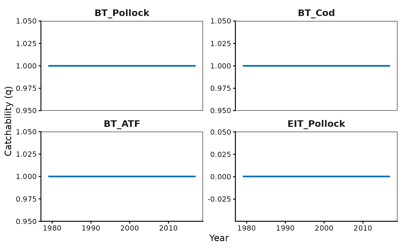
Plots the fitted survey catchability q by year, faceted by fleet. Every
fleet holding index_data is drawn, a fishery with a CPUE series as much as
a survey.
Usage
plot_catchability(
  Rceattle,
  file = NULL,
  model_names = NULL,
  species = NULL,
  spnames = NULL,
  mse = FALSE,
  minyr = NULL,
  maxyr = NULL,
  incl_mean = FALSE,
  log = FALSE,
  line_col = NULL,
  lwd = 3,
  lty = 1,
  width = 7,
  height = 6.5,
  right_adj = 0,
  top_adj = 0.05,
  single.plots = FALSE
)
Arguments
- Rceattle
A single
fit_mod()object or a list of them (overlaid).- file
Optional file stem; the figure is written to
<file>_<suffix>.pngif given.- model_names
Legend labels for the models.
- species
Species to include, as indices (
c(1, 3)), names, a logical mask, or"all". DefaultNULLplots every species. Species labels belong inspnames; a characterspeciesthat matches no species name is read as labels for back-compatibility.- spnames
Species labels, length
nspp. Default: the model's own.- mse
Is
Rceattlean MSE object? Its operating models are drawn.- minyr, maxyr
First / last year to plot.
- incl_mean
Add a horizontal line at the hindcast mean of each series.
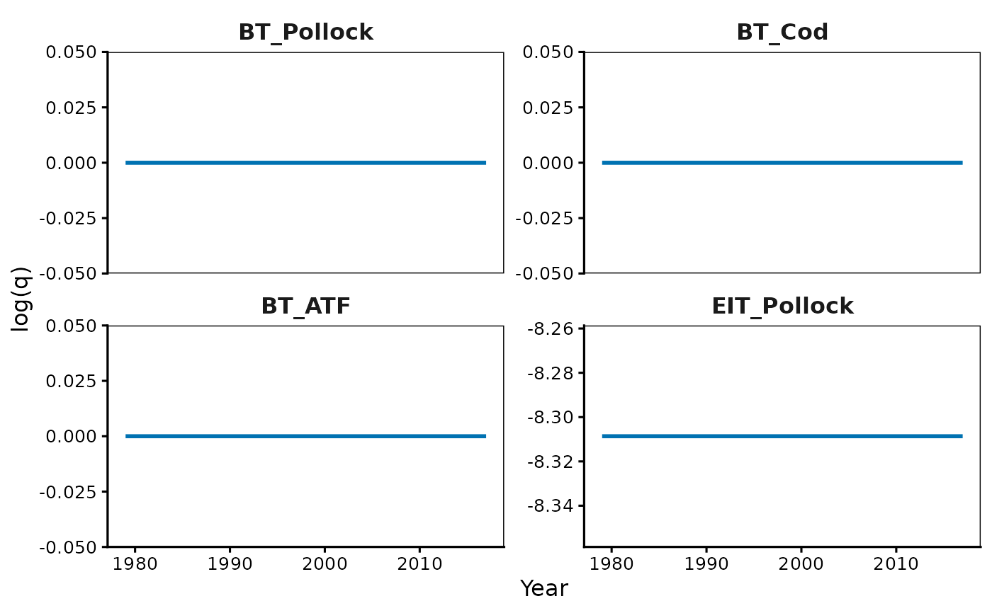
- log
Plot catchability on the log scale.
- line_col
Line colours; names, hex, or base-graphics integers.
NULLuses the colorblind-safe Okabe-Ito palette. Applied to whichever variable the figure separates by colour, in legend order. Too few colours are recycled, with a warning.- lwd
Line width on the base-graphics scale: the default
3renders as a standard-weight ggplot line. A vector varies it across series.- lty
Line type. A vector varies it across the levels of whatever the figure separates by line type.
- width, height
Saved figure size in inches.
- right_adj
Ignored. Base-graphics leftover: the figure widened its right margin to fit the legend. Set margins on the returned ggplot instead.
- top_adj
Ignored. Base-graphics leftover; see
right_adj.- single.plots
Ignored. Base-graphics leftover: one device per panel. The ggplot facets instead.
Details
The value plotted is the realized catchability the model scaled the survey by,
whichever route produced it: an estimated or fixed mean, annual deviations
under Time_varying_q, an environmental regression (Catchability = "Environmental"), a q linkage such as rw(1 | Year) or ar1(1 | Year), or
the closed-form value under "Analytical" / "AnalyticalArith". A fleet with
a time-invariant catchability draws a flat line, which is the honest picture
of a constant q rather than an empty panel.
Hindcast years only. The model applies catchability over the hindcast and
does not project it, so the series stops at endyr regardless of the
projection horizon. There is no incl_proj.
line_col and lty separate the models, so overlaying several fits
compares their catchability series panel by panel.
Examples
# \donttest{
data(BS2017SS)
fit <- Rceattle::fit_mod(data_list = BS2017SS, msmMode = 0)
#> `age_trans_matrix` data does not span range of age for species 1 will fill with 0s
#> Step 1: Parameter build complete
#> Step 2: Map build complete
#> Step 3: Parameter bounds complete
#> Step 4: Data rearrange complete
#> Step 5: Hindcast build complete
#> Step 6: Hindcast optimization complete
plot_catchability(fit)
 plot_catchability(fit, log = TRUE)
 # }