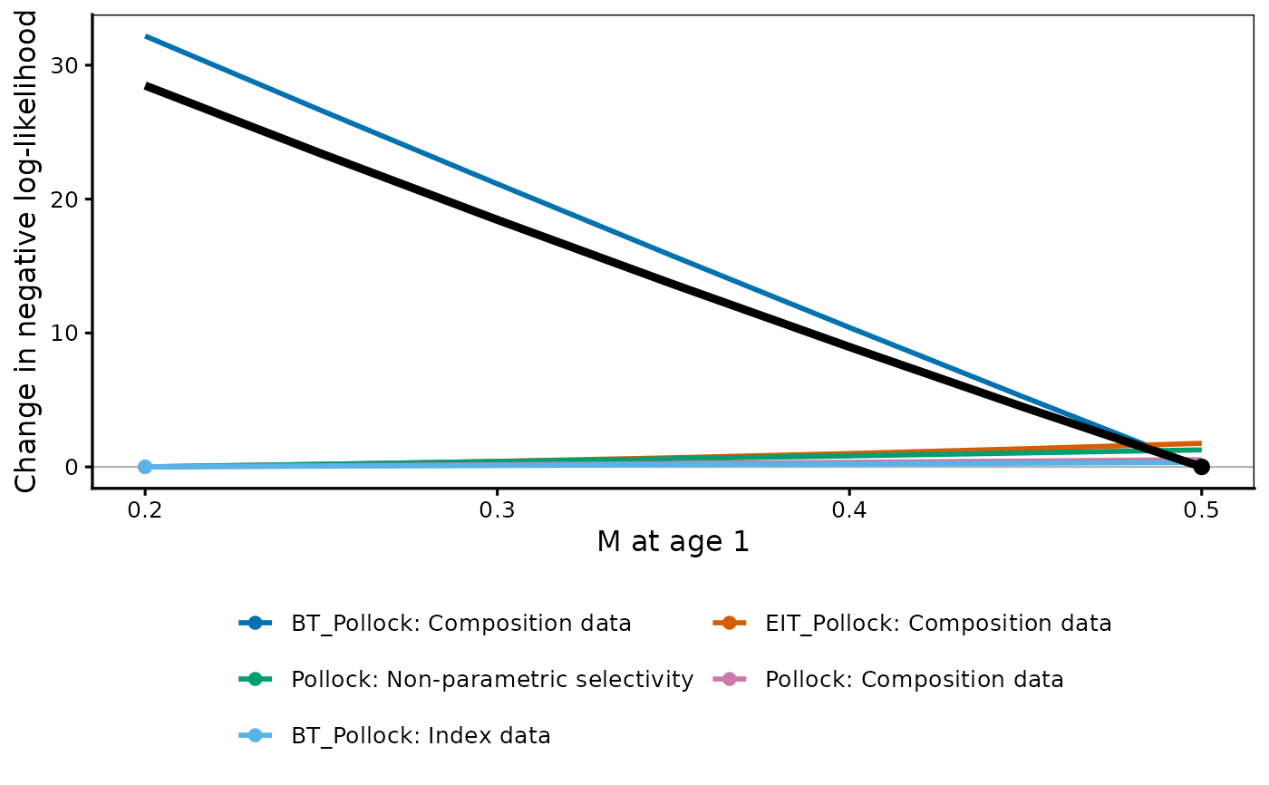
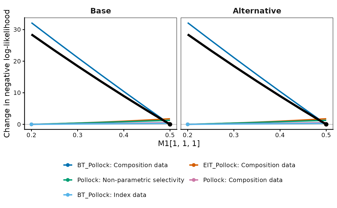
Plot the likelihood components across a profile

Draws each negative log-likelihood component against the profiled parameter, with the total overlaid, in the style of r4ss::SSplotProfile(). Where the curves disagree about which value they prefer, the data sources are in conflict, which is what the total on its own cannot show.

Usage

plot_profile(
  Rceattle_profile,
  model_names = NULL,
  weighted = TRUE,
  relative = c("own", "scaled", "minimum", "none"),
  minfraction = 0.01,
  add_cutoff = FALSE,
  cutoff = 1.92,
  xlab = NULL,
  ylab = NULL,
  line_col = NULL,
  lwd = 3,
  lty = 1,
  file = NULL,
  width = 7,
  height = 5
)

Arguments

Rceattle_profile: A single "Rceattle_profile" from profile.Rceattle(), or a list of them to compare models in facets.
model_names: Legend labels for the models.
weighted, relative, minfraction: Passed to profile_components(), which documents them. minfraction defaults to 0.01 here, as in r4ss::SSplotProfile().
add_cutoff: Draw a horizontal line at cutoff. Off by default: the cutoff is a statement about the total, and drawing it across the components invites reading it as one about them.
cutoff: Height of that line. Default 1.92, the 95% profile-likelihood cutoff for one parameter, $\chi^2_1(0.95)/2$.
xlab: X-axis label. Default names the profiled parameter and cell in the units the grid is in.
ylab: Y-axis label. Default follows relative.
line_col: Line colours; names, hex, or base-graphics integers. NULL uses the colorblind-safe Okabe-Ito palette. Applied to whichever variable the figure separates by colour, in legend order. Too few colours are recycled, with a warning.
lwd: Line width on the base-graphics scale: the default 3 renders as a standard-weight ggplot line. A vector varies it across series.
lty: Line type. A vector varies it across the levels of whatever the figure separates by line type.
file: Optional file stem; the figure is written to <file>_<suffix>.png if given.
width, height: Saved figure size in inches.

Value

A ggplot object. Its $data is the plotted frame, so the numbers behind the figure can be read back off it.

Details

Read the figure by where each curve bottoms out, not by how deep it is. Every series is re-zeroed at its own minimum and a point marks that minimum, so the spread of the points along the x axis is the disagreement: components whose points sit together support the same value, and one whose point sits far from the total's is pulling against the rest. Where one component dwarfs the others it sets the y axis and the rest flatten onto the bottom; relative = "scaled" puts every curve on 0 to 1 so the minima stay comparable, and relative = "minimum" re-zeroes every series at the total's minimum, showing what each gives up by moving away from the fitted value. profile_components() documents all of them, and the magnitude "scaled" discards.

The total is drawn solid and black at 1.6 times lwd, and kept out of the colour legend, so it stays the reference line whatever the components are styled as; line_col, lwd and lty therefore apply to the components. Series are ordered, in the legend and the palette, by how much each moves over the grid. Under joint = "multiply" or "add" a dotted vertical line marks the fitted model (a multiplier of 1, an offset of 0). Non-converged grid points leave a gap.

References

Taylor, I.G., et al. (2021) Beyond visualizing catch-at-age models: Lessons learned from the r4ss package about software to support stock assessments. Fisheries Research 239: 105924.

Examples

# \donttest{
data(BS2017SS)
ss_run <- fit_mod(data_list = BS2017SS, inits = NULL, file = NULL,
    estimateMode = 0, random_rec = FALSE, msmMode = 0, avgnMode = 0,
    phase = FALSE, verbose = 0)
#> Warning: Passing ‘phase’, ‘verbose’ directly to fit_mod() is deprecated and will be removed in a future release. Bundle these into fit_control() instead, e.g. fit_control(phase = ..., verbose = ...). Forwarding for now.
#> `age_trans_matrix` data does not span range of age for species 1 will fill with 0s

# Profile M for species 1 and see which data sources disagree about it
prof <- profile(ss_run, param = "M1", slots = list(c(1, 1, 1)),
                values = list(seq(0.2, 0.5, by = 0.05)))

plot_profile(prof, xlab = "M at age 1")


# Two model configurations side by side
plot_profile(list(prof, prof), model_names = c("Base", "Alternative"))

# }