Greenland turbot: a fully worked example • spmR

Fully worked example

Download the fully worked example to get the actual ForProjections.dat, spm.dat and tacpar.dat files, a plain-language field guide, installation requirements, and a short R script for checking or changing inputs, running a new attempt, plotting selected alternatives and exporting useful CSV tables. The bundle includes one completed conditional run and its provenance; new runs preserve it.

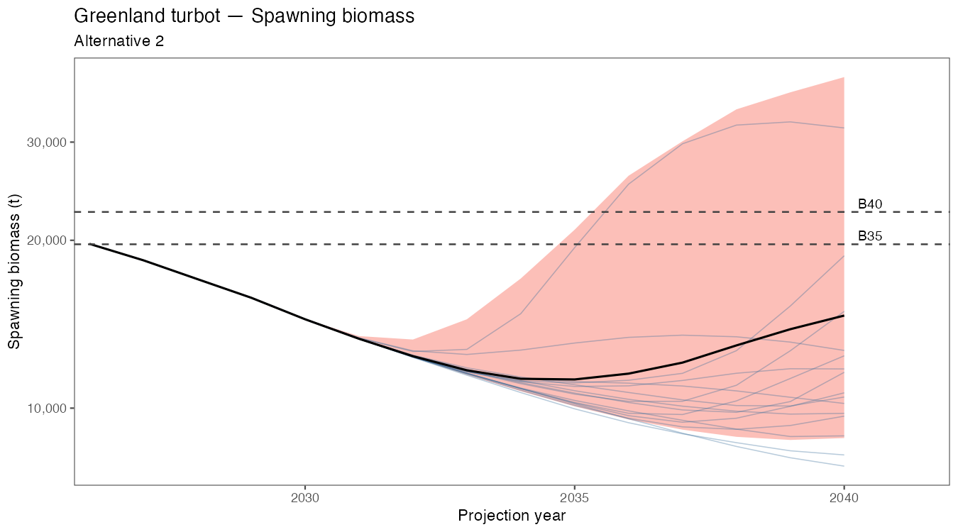
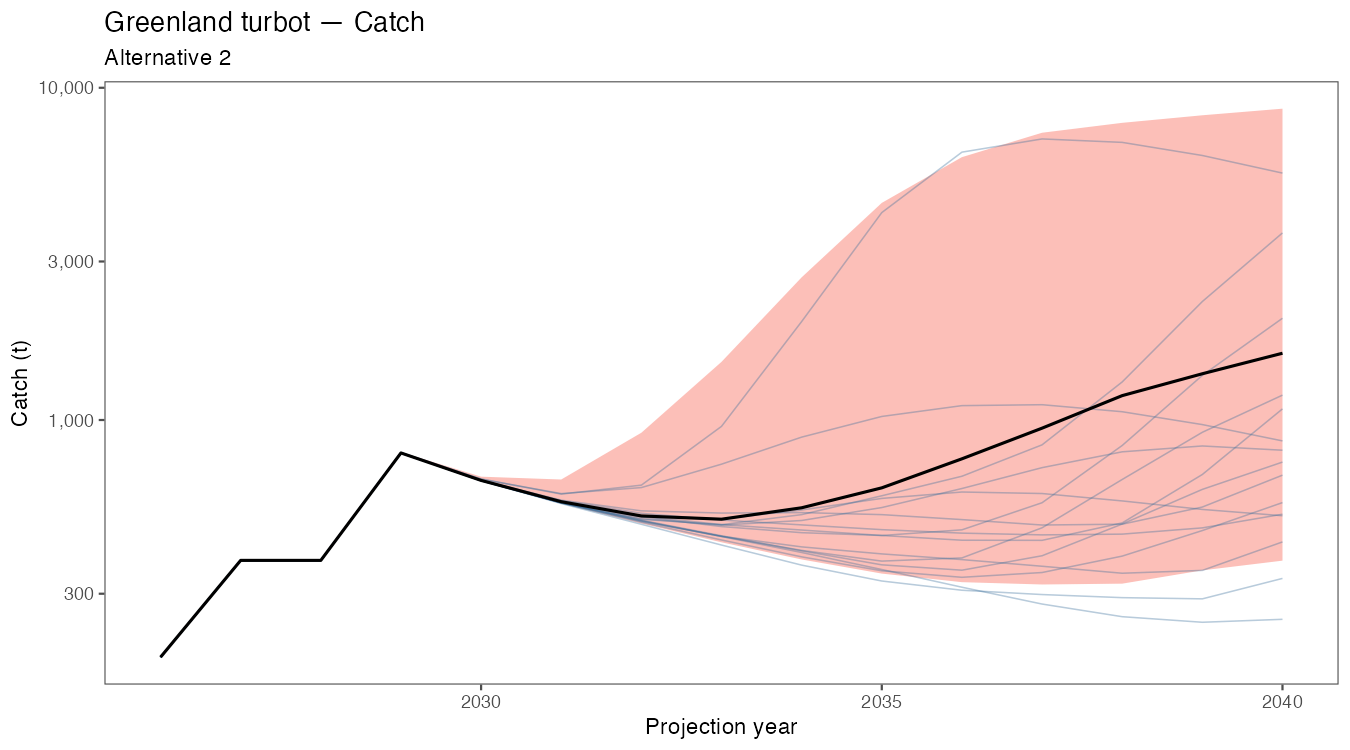
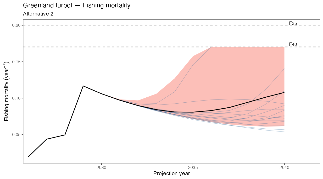
Open the rendered Greenland turbot results for three Alternative 2 figures: spawning biomass and catch on logarithmic y-axes, and fishing mortality on a linear y-axis. Dashed reference lines show B40 and B35 on the spawning-biomass figure and F35 and F40 on the fishing-mortality figure. Salmon ribbons show the 90% projection intervals. This example uses Jim’s confirmed local 47-value SSB history and diagnostic population-weight assumptions; successful execution is separate from scientific input review. Figure downloads: spawning biomass, catch, and fishing mortality.

The examples/gt_2026 directory preserves the supplied Greenland turbot projection files. The current species input contains 47 recruitment values and 47 SSB values. The counts match; their calendar alignment still requires confirmation. Population body weights, units, age and plus-group alignment, and SS3 export-field mapping also require confirmation before assessment use. This article executes a read-only audit; it stages no files and generates no projection results.

Simple commands

Install the current spmR package and work from a clone of the source repository. From its root:

source("examples/gt_2026/run.R")
check_gt2026_inputs()

The audit reads the current source values. Confirm the recruitment and SSB histories and their year alignment before staging. diagnostic = TRUE selects working population weights, units and ages explicitly; it cannot supply missing history values or establish their calendar alignment. Once inputs are reviewed, each successful default staging call creates examples/gt_2026/spmR_runs/attempt-###, retaining source snapshots, SHA-256 hashes, embedded declarations, and staging decisions. Existing attempt directories are protected against overwriting.

Audit the supplied files

The article locates and audits the example during its build. It requires the source checkout or source package, where the example files are available.

audit <- check_gt2026_inputs(example_dir)
gt::gt(audit)

item	status	detail
Native metadata	info	A separate spm_input_v2.dat is optional; the runner embeds validated declarations in the staged species file.
R metadata	info	A separate spm_metadata.json is optional. Existing files are archived; staged declarations come from explicit arguments or diagnostic defaults.
Recruitment rows	repair	2 copies of a 47 value series across 2 lines; retain one complete series. A second copy would be read as SSB.
Recruitment basis	ok	Source explicitly declares per_sex recruitment.
Spawning weights	repair	4 zeros in effective spawning weights; stage them as 1e-12 for the current positive-weight contract.
Population weights	missing	Population body weights require explicit runner arguments and SS3 verification. Diagnostic defaults use Fratio-weighted catch-weight proxies, with fleet fractions 0.96, 0.04
Units and ages	review	Thousand fish, kg, tonnes and ages 1:30/30+ are working assumptions requiring SS3 export verification.
SSB history	review	47 positions; source label: # SSB 1978-2026 . Calendar pairing remains unresolved; restrict to Tier 3, Rec_Gen=1. The final two SSB values repeat the preceding pair; confirm this with the source export.
Maturity fields	info	All-one maturity retains effective spawning weights. Ntot and SexRatio describe all fish and the all-fish female fraction. Confirm the SS3 spawning-weight definition.
Controls	ok	2026-2040; 7 alternatives; 1000 simulations. Adapter requires Tier 3, Rec_Gen=1, TAC_ABC=1, beginning year 2026 and ForProjections.dat.
TAC parameters	info	tacpar.dat is archived when supplied and unused with TAC_ABC=1.

The input recruitment basis is per_sex. It contains 2 recruitment copies with 47 values each across 2 numeric lines, ending in 811.8, 460.5. The SSB series ends in 28053.3, 27020.6, 25862.1, 27020.6, 25862.1. The final two SSB values repeat the preceding pair. Confirm that these are the intended source values rather than placeholders.

The source history labels are printed below. Counts alone establish neither the calendar years nor the recruitment/SSB year pairing. Confirm both against the SS3 export, including any labels that remain from an earlier revision.

cat(history_labels, sep = "\n")

# Recruitment 1978 to 2022 for RecAge=1
# SSB 1978-2026

The helper accepts wrapped recruitment series and an explicit basis. With matching source histories and declared inputs, it can stage one recruitment copy, move the basis declaration into the versioned comment block, and replace four zero spawning weights with 1e-12 for the positive-weight contract. It keeps Tier 3 historical-recruitment mode (Rec_Gen = 1). That mode still requires matching positional recruitment and SSB lengths.

The obsolete placeholder sidecar was removed from the canonical example; earlier source snapshots remain archived. Separate JSON and native metadata files are optional in version 0.4.3: the helper writes validated declarations as comments in the staged species file. The current native engine reads those comments directly. spm.tpl is self-contained and requires no separate C++ header.

Check staging readiness

The following table selects the current findings that need repair, declarations, or review. It reads the audit without choosing diagnostic assumptions or creating an attempt directory. The runner can repair duplicate recruitment copies and zero spawning weights during staging; population weights, units, and ages require explicit arguments or an explicit diagnostic choice. Calendar alignment and the SS3 field definitions require scientific review in either case.

readiness <- audit[audit$status %in% c("missing", "review", "repair"), ]
readiness |>
  dplyr::rename(
    readiness_item = item,
    readiness_status = status,
    readiness_detail = detail
  ) |>
  gt::gt() |>
  gt::cols_label(
    readiness_item = "item",
    readiness_status = "status",
    readiness_detail = "detail"
  )

item	status	detail
Recruitment rows	repair	2 copies of a 47 value series across 2 lines; retain one complete series. A second copy would be read as SSB.
Spawning weights	repair	4 zeros in effective spawning weights; stage them as 1e-12 for the current positive-weight contract.
Population weights	missing	Population body weights require explicit runner arguments and SS3 verification. Diagnostic defaults use Fratio-weighted catch-weight proxies, with fleet fractions 0.96, 0.04
Units and ages	review	Thousand fish, kg, tonnes and ages 1:30/30+ are working assumptions requiring SS3 export verification.
SSB history	review	47 positions; source label: # SSB 1978-2026 . Calendar pairing remains unresolved; restrict to Tier 3, Rec_Gen=1. The final two SSB values repeat the preceding pair; confirm this with the source export.

Stage complete inputs after review

Diagnostic mode uses 0.96 × fleet 1 + 0.04 × fleet 2 catch-weight proxies separately for each sex as population weights. These coefficients are the supplied fishing-mortality allocation. The mixture is a computational assumption and requires review as a representation of population body weight. Diagnostic mode also declares thousand fish, kg, tonnes, and ages 1–30 with a terminal plus group. Whether the supplied spawning weights already incorporate maturity requires confirmation; the all-one maturity fields are neutral multipliers. Under those fields, Ntot and SexRatio describe all fish and the all-fish female fraction.

staged <- run_gt2026_projection(
  source_dir = example_dir,
  run_dir = tempfile("spmr-gt2026-article-"),
  diagnostic = TRUE,
  run = FALSE
)
staged$run_dir

This command is displayed without execution. It requires matching source histories and an explicit decision to use the diagnostic assumptions.

Run an explicitly chosen diagnostic projection

After confirming the histories and explicitly choosing the diagnostic assumptions, these commands enable native execution. They are displayed without execution in this article.

gt2026 <- run_gt2026_projection(diagnostic = TRUE)
gt2026$summary
gt2026$run_dir

The helper uses admb on PATH, SPMR_ADMB, or its admb argument to compile the installed template. SPMR_CXX selects a matching C++ compiler. A compatible existing executable can be selected with SPMR_EXECUTABLE or executable. If compilation still requests spmr_input_v2.hpp, reinstall spmR from the current checkout and restart R to refresh the installed template.

A completed run under the supplied controls would contain 105,000 detail rows: seven alternatives, 1,000 simulations, and 15 projection years (2026–2040). The helper verifies the row keys, finite outputs, initial biomass, fixed catches, and successful provenance. Gradient and Hessian fit diagnostics are inapplicable to historical-recruitment simulation. These checks establish the conditional calculation; the SS3 export definitions and scientific interpretation require their own review.

Replace the population-weight assumptions

Provide actual female and male population body-weight vectors with verified units and age labels:

gt2026 <- run_gt2026_projection(
  population_weights = list(
    female = female_body_weights,
    male = male_body_weights
  ),
  units = verified_units,
  ages = verified_ages
)

Each vector must align with the 30 supplied age positions. Confirm the beginning-of-2026 abundance state, plus group, and recruitment/SSB year pairing against the SS3 export code and source fields. Supplying population weights alone leaves those remaining checks open. The example README contains the complete input evaluation and terminal commands.

Standalone run-and-results report

examples/gt_2026/greenland_turbot.qmd provides visible manual run controls, the current input audit, and three Alternative 2 figures. Spawning biomass and catch use logarithmic y-axes; fishing mortality uses a linear y-axis. Dashed reference lines show B40 and B35 on the spawning-biomass figure and F35 and F40 on the fishing-mortality figure. All three figures show the all-simulation median and a salmon 90% projection interval. Rendering performs no projection; select a reviewed saved attempt to populate the results. From the repository root:

quarto render examples/gt_2026/greenland_turbot.qmd
quarto render examples/gt_2026/greenland_turbot.qmd -P saved_run:spmR_runs/attempt-001

The first command produces the audit only, including in a fresh source checkout without saved output. The second selects results explicitly.

Replace attempt-001 with the intended saved attempt. Saved results from an older source revision are labelled separately from the current input audit.