A basic example showing how to use afscISS for a
production run.
library(afscISS)
#> Loading required package: data.table

# set some globals
species = c(30150, 30152) # dusky rockfish
region = 'goa'
comp = 'length'
sex_cat = 4 # post expansion
spec_case = 'dr' # dusky rockfish is a special case
Plot the length composition ISS.
plot_ISS(species = species,
         region = region,
         comp = comp,
         sex_cat = sex_cat,
         spec_case = spec_case)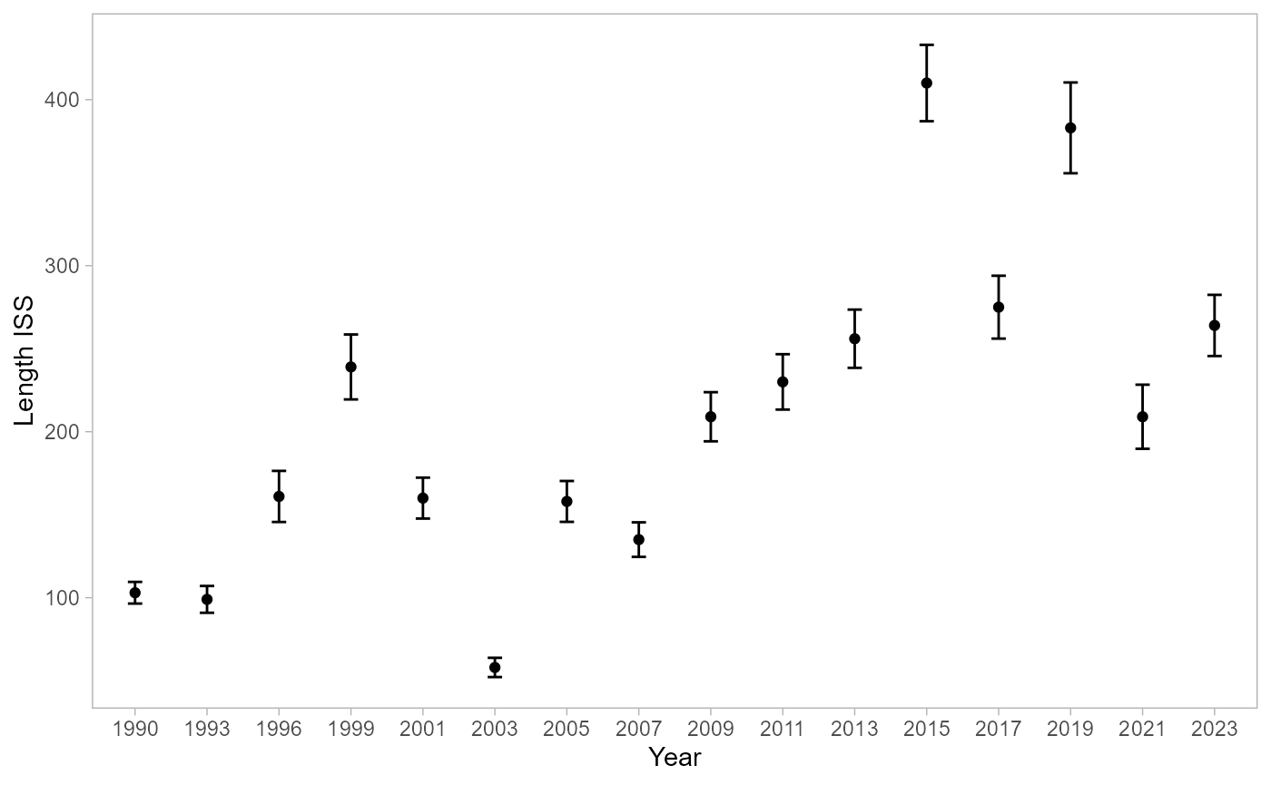
Get the length composition data frame.
get_comp(species = species,
         region = region,
         comp = comp,
         sex_cat = sex_cat,
         spec_case = spec_case)
#> # A tidytable: 557 × 8
#>     year species_code   sex sex_c length     prop q2_5th q97_5th
#>    <dbl>        <dbl> <dbl> <dbl>  <dbl>    <dbl>  <dbl>   <dbl>
#>  1  1990       301502     4     4     22 0.00808       0 0.0336
#>  2  1990       301502     4     4     23 0.00404       0 0.0163
#>  3  1990       301502     4     4     24 0.00202       0 0.00962
#>  4  1990       301502     4     4     25 0.00606       0 0.0221
#>  5  1990       301502     4     4     27 0.00649       0 0.0256
#>  6  1990       301502     4     4     28 0.00606       0 0.0227
#>  7  1990       301502     4     4     29 0.00657       0 0.0237
#>  8  1990       301502     4     4     31 0.00102       0 0.00472
#>  9  1990       301502     4     4     32 0.00692       0 0.0237
#> 10  1990       301502     4     4     33 0.000736      0 0.00324
#> # ℹ 547 more rows
Examine the same items for age composition data.
plot_ISS(species = species,
         region = region,
         comp = 'age',
         sex_cat = sex_cat,
         spec_case = spec_case)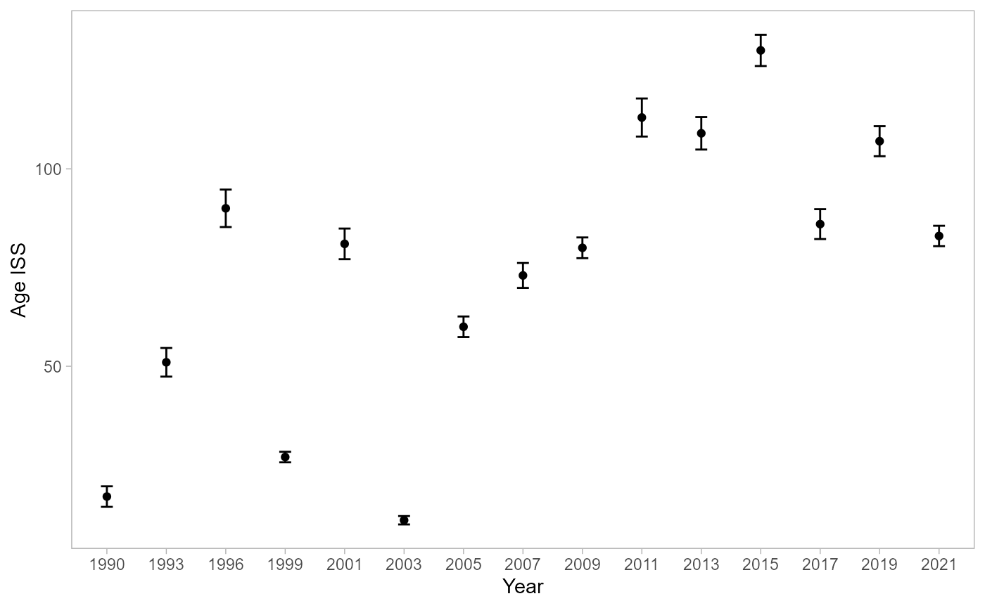
Get the age composition data frame.
get_comp(species = species,
         region = region,
         comp = 'age',
         sex_cat = sex_cat,
         spec_case = spec_case)
#> # A tidytable: 511 × 8
#>     year species_code   sex sex_c   age    prop   q2_5th q97_5th
#>    <dbl>        <dbl> <dbl> <dbl> <dbl>   <dbl>    <dbl>   <dbl>
#>  1  1990       301502     4     4     6 0.00263 0        0.0162
#>  2  1990       301502     4     4     7 0.00103 0        0.00433
#>  3  1990       301502     4     4     8 0.00107 0        0.00427
#>  4  1990       301502     4     4     9 0.00813 0.000727 0.0338
#>  5  1990       301502     4     4    10 0.108   0.00337  0.378
#>  6  1990       301502     4     4    11 0.131   0.00460  0.318
#>  7  1990       301502     4     4    12 0.112   0.0130   0.285
#>  8  1990       301502     4     4    13 0.152   0        0.328
#>  9  1990       301502     4     4    14 0.200   0.0414   0.406
#> 10  1990       301502     4     4    15 0.100   0.0107   0.263
#> # ℹ 501 more rows