
Eastern Bering Sea walleye pollock stock assessment
September 2024
Executive Summary
Summary of Changes in Assessment Inputs
The work presented below was based on the same data sets used in the 2023 assessment. The model was updated so that it could handle a number of requests from the SSC. We enhanced the capability of the code to deal with some alternative hypotheses of factors that affect the stock recruitment relationship (SRR). We stepped through a number of sensitivity analyses to evaluate the stock-recruitment relationship (SRR) and the steepness of the SRR. We also evaluated the impact of including the natural mortality-at-age estimates from CEATTLE model.
Summary of Results
Some research has indicated that the value of \(\sigma_R\) can be reasonably well estimated in both traditional stock assessment models and in state-space versions (e.g., Stock and Miller (2021)). Based on our analysis, we confirm that estimates appear reasonable. However, we caution about applying \(\sigma_R\) estimates blindly in management settings. This is because for EBS pollock, the SRR is heavily influenced by estimates of spawning biomass being mainly larger than \(B_{MSY}\) (to the right of \(B_{MSY}\); far from the origin of the SRR curve) instead of spawning biomass estimates that are much smaller than \(B_{MSY}\) (near the origin, which would better inform estimates of steepness). We show that the SRR is thus linked to the Tier 1 fishing mortality recommendation in two ways: 1) by the assumption about \(\sigma_R\) (smaller values increase the “precision” of \(F_{MSY}\)) and 2) by having most of the data far from the origin means estimating steepness becomes less certain and possibly unreliable. We provided an illustration of this in an external simulation. In the 2023 assessment, \(\sigma_R\) was specified at 1.0 as a precautionary measure. We seek guidance on \(\sigma_R\) approaches and general treatment of the SRR given the direct management implications under Tier 1.
Incorporating the natural mortality-at-age and year from CEATTLE had a modest impact on the SRR because the recruitment scales were higher.
The model code was updated to work as an operating model so that a full-feedback simulation loop could be used to test different management procedures.
Presently the ecosystem factors that affect the pollock TAC are mostly related to the constraint due to the 2-Mt cap. We attempt to elaborate more directly on the ecosystem aspect by developing a parallel catch guideline that is intended to take into account the role pollock plays in the ecosystem. We contrast this alternative guideline (in the form of “advice”) with historical patterns of catch. Additionally, we consider multi-species mass-balance projections under scenarios where catch projections closer to the maximum permissible are used. This was done using “ecosense” within the package Rpath (Aydin, Lucey, and Gaichas (2024); courtesy Andy Whitehouse).
Responses to SSC and Plan Team Comments
From the 2023 SSC minutes:
The SSC would prefer not to make a risk table adjustment based on the difference from Tier 1 to Tier 3 again during the 2024 assessment cycle. The SSC requests that the next stock assessment bring back a new approach that may include development of a constant buffer based on factors extrinsic to the stock assessment (ecosystem function), or a better representation of the uncertainty in the Tier 1 and control rule calculations such that a reduction from maximum ABC is not needed every year.
- We approached this by first examining the stock recruitment relationship (SRR) and review the assumptions that the SSC has used to classify this stock in Tier 1 of the BSAI FMP. This is covered under a separate request by the SSC detailed below. We also attempted to consider factors that explicitly acknowledge the importance of pollock to the EBS ecosystem. We propose a management procedure that provides stability in the ABC advice each year and tracks historical adjustments as needed during periods of spawning biomass declines below target (where here we propose using a target geared towards 40+ years of experience managing this fishery).
Use posterior distributions from the MCMC to determine probabilities in the risk table and expand the columns in the risk table to include the recommended ABC (and potentially higher values).
- We interpret this request to refer to the decision table included in the assessment and not the risk-table that is standardly produced for all groundfish assessments. Using the posterior distributions to compute probabilities requires some simple code modifications. Since previous results indicated that asymptotic approximations performed similarly near the mode, we had used them as a shortcut method to make the decision table.
Identify where MLE estimates are being used and where MCMC estimates are being used. Also see the SSC’s General Stock Assessment Comments to include convergence diagnostics any time Bayesian results are reported. If MCMC diagnostics continue to appear adequate, reference points could be calculated using the posterior distribution used, rather than an analytical calculation.
- MLE and asymptotic approximations have always been used for advice. Results from sampling the posterior distribution have been used as a comparison and to show inter-relationships. This will require some document-code modifications to do the computations off of the posterior distributions
The SSC recommends that consideration be given to removal of the Japanese fishery CPUE index (1965-76) from the assessment, because this data set no longer seems to contribute to the assessment. A sensitivity test should be done to evaluate the effects of data removal on the assessment.
- We investigated this and report on it here.
Catch-at-age data provided by foreign fishing agencies in the pre-Magnuson era were not produced using the same aging criteria as the AFSC age-and-growth program. Consideration should be given to removal of these data from the assessment. A sensitivity test should be done to evaluate the effects of data removal on the assessment.
- We investigated this and report on it here.
Document the method used for determining the selectivity to use in the forward projections and continue to evaluate projection variability due to selectivity. The SSC appreciates the selectivity retrospective comparison and suggests that it might be helpful to limit the comparison to the projection used in each year against only the most recent (best) estimate of selectivity for that year.
- We will be clearer about projection assumptions especially for selectivity. In this report we show the sensitivity of selectivity assumption and evaluated the sensitivity of Tier 1 ABC estimates given different selectivity estimates from historical annual values. In the next draft we will update how different selectivity assumptions perform based on an updated retrospective presentation for this year’s assessment.
The SSC supports the use of posterior predictive distributions, an underutilized tool in fisheries science, but common in other fields. To fully implement this approach to Bayesian model checking the SSC recommends plotting a histogram for each data source of the percentile of the predictive distribution in which each data point lies, noting that in a highly consistent model this histogram would be uniform.
- In Bayesian statistics, evaluating the performance of a model using the percentile of the posterior predictive distribution is a common approach. This process involves comparing observed data to predictions made by the model and we understand the calculations that would be needed but have yet to implement the necessary code. We highlight the approach in a section discussing Bayesian diagnostics in this report.
There is an apparent shift towards older ages in fisheries and trawl survey selectivity that should be investigated further.
- This is illustrated in the selectivity plots presented in last year’s report. Relative to historical estimates, the shift seems consistent with past years.
The SSC agrees with the BSAI GPT’s proposal in their presentation to move the multi-species model out of the pollock stock assessment, where it has been included as an appendix since it was first developed. Instead, they suggested it would be a separate chapter listed in parallel with the ESR, as it applies to multiple stocks and informs the ESRs.
- Technically it’s presented as part of the BSAI assessment. Agree that it should be highlighted on its own. In this report we included the age and year specific estimates of natural mortality from CEATTLE.
The SSC suggests revisiting the treatment of the stock-recruit relationship in the assessment model using recent improvements in modeling approaches and a longer time series that encompasses the recent warm period in the EBS. Recruitment deviates should be from the stock-recruit relationship and should model variability among annual recruitment estimates based on information in the data and residual variability. The estimation process should ensure that log-normally distributed recruitments are mean unbiased, resulting in unbiased biomass estimates. If an informative prior is used for steepness, it should be based on a meta-analysis of related species and reflect the uncertainty of that meta-analysis. Further consideration of time periods (as in previous analyses) and the influence of temperature on the stock-recruit relationship may be helpful. The SSC recognizes that there were significant recent analyses in 2016, 2018 and 2020 and is not requesting a repeat of those but a review of previous work would be helpful.
- We examine a model where the SRR applies over all age classes along with a reevaluation of a number of factors that affect the SRR and the \(F_{MSY}\) values. We include a few model results where temperature is in the condition of the SRR. We also note that an evaluation of different ‘regimes’ or periods of low or higher recruitment has been presented in the standard assessment for several years (maybe decades?).
Stock-recruit relationship sensitivities
As noted, in the previous section, the SSC asked for a more detailed review of how the SRR was implemented. This included a review of the assumptions about the SRR.: We attempt to address this in the subsequent sections. For backgound, the FMP specifies that the SSC’s criterion for Tiers 1 and 2 ABC/OFL estimates depend on having reliable estimates of \(F_{MSY}\). For this reason, the stock-recruitment relationship (SRR) is a key component of the advice. Over the years, we have compared different aspects of the SRR assumptions. The SSC requested a further evaluation and recap of what has been done previously. The following aspects of the SRR were evaluated and reviewed this year
- Selectivity
- Time series length
- Temperature
- Priors (on steepness)
- Form (e.g., Ricker versus Beverton-Holt)
- \(\sigma_R\)
We also examined some inverse relationships relative to the SRR. For example, the model can fit a curve that satisfies conditions such as
- what curve best fits the data yet satisfies the constraint that \(F_{MSY}\) is equal to \(F_{35\%}\)
- what curve best fits the data yet satisfies the constraint that \({MSY}\) is equal to the historical mean (e.g., the long-term mean of 1.3 million t)
Time series length for the stock-recruitment relationship conditioning
The SSC requested that the full time series be included for the SRR conditioning. Extending the time series back to 1964 resulted in a different shaped curve with higher steepness (Figure 1). This was due to the inclusion of age-1 recruits from the early years. The inclusion of sea-surface temperature as a covariate to the full time series moderated this increase slightly (Figure 2).

Stock recruitment relationship estimates with different terminal years
An alternative SRR conditioning exercise was conducted where the year range for the conditioning of the curve was dropped in successive years. This was intended to show how sensitive the curve is to the years included in the analysis. We expect that it should revert to the prior as fewer years are included in the conditioning of the SRR curve. To consider the variability of the SRR estimates due to additional years of data, we changed the window of years used within the assessment model. Results showed given the prior and other assumptions, the SRR estimates were relatively stable (Figure 3 and Figure 4).

Removing the impact of the prior on the stock-recruitment relationship
As we have done in past years, we evaluated the impact of the prior on the SRR. Results indicate that without the prior on steepness the estimate increases dramatically (Figure 5). For this case the estimate of \(B_{MSY}\) drops to nearly half of the status quo value (and below most of the historical estimates of spawning biomass). The fishing effort to achieve \(F_{MSY}\) in this case would be much higher than the current Tier 1 estimates. From a management perspective, this would be a significant change in the advice and one poorly founded on actual experience.

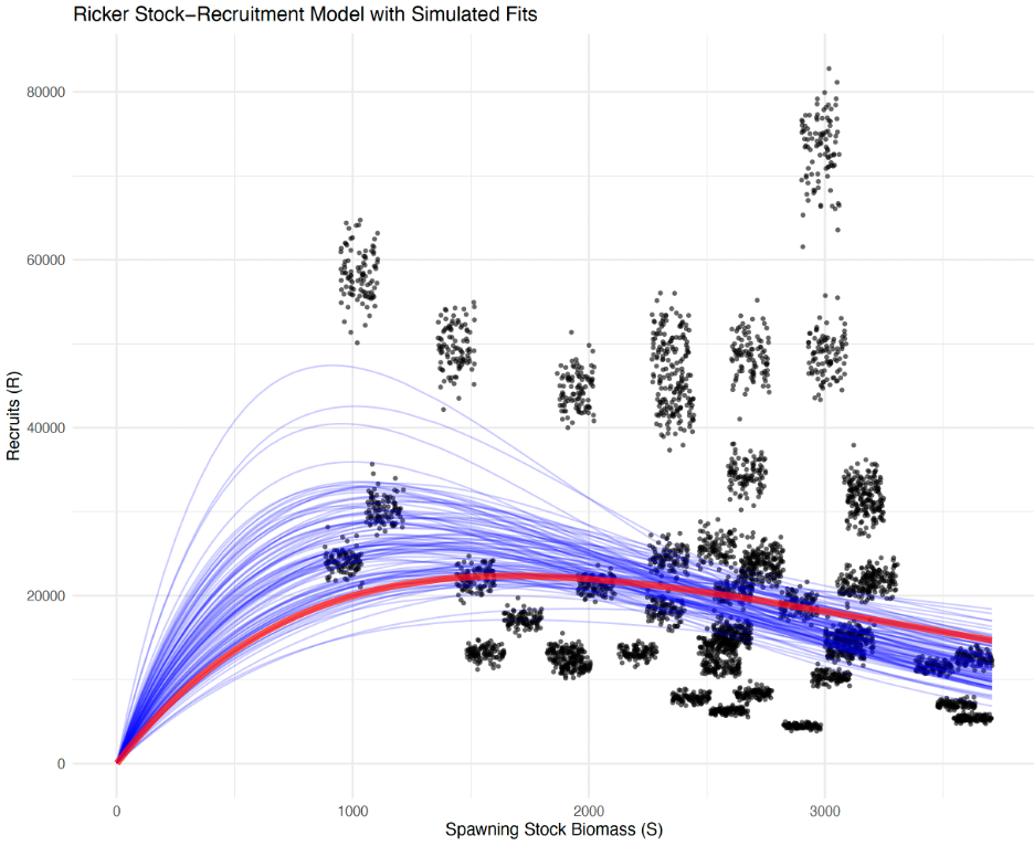
Simulation testing the stock recruitment estimation
A simple simulation framework was set up to show how patterns of the Ricker SRR can be influenced by the available “points” used in the estimation. We start with the estimates of spawning biomass and recruits from the 2023 accepted model. As in the assessment, we selected the period from 1978-2022 and fit a Ricker SRR. We then replicated the estimation using random error about both the estimate of recruitment and spawning biomass. These “data” were then sampled with replacement. The
100 sets of data and resulting curves showed that the slope at the origin tends to be higher for these cases (are shown in (Figure 6). Note that these curves differ from the actual assessment since the fitting is done separately (we used the linear regression log recruits-per-spawning biomass vs spawning biomass). The point of this exercise is to show that extrapolating the fitted curves outside of the range of data (i.e., at smaller spawning stock sizes) can lead to very different and positively biased productivity estimates. The slope at the origin is a key parameter in the Ricker SRR and governs productivity estimates and consequently, \(F_{MSY}\) estimates. This suggests that applying the SRR estimates for management purposes (in Tier 1) may be inappropriate given this apparent potential for bias.
Beverton-Holt stock-recruitment relationship
Traditionally the SRR form has been parameterized as a “Ricker” due to the presence of cannibalism. As part of the review of different approaches for modeling the stock-recruit relationship, we compared last year’s model with different forms, priors, and periods using the Beverton-Holt curve. The shorter and longer periods with the Beverton-Holt curve (using the same priors) were similar to the Ricker curve, but had higher uncertainty (Figure 7). Removing the prior on the Beverton-Holt curve resulted in estimates of steepness near 1.0 and higher precision (Figure 8).


Specified variability about the SRR
The SSC requested that we ensure that the bias correction is applied in the application of fitting the SRR. We confirm that in past assessments, for the period which the SRR curve was applied, the bias correction term was included. Specifically,
\[ \hat{R}_t = f(B_{t-1}) e^{\epsilon_t-0.5 \sigma_R^2} \]
where \(\epsilon_t \sim N(0, \sigma_R^2)\). Here the production function (which generates age-1 recruitment) is a function of spawning biomass in the previous year (\(f(B_{t-1})\)). Since this function “generates” age-1 recruitment from a lognormal distribution, the basis for this must be scaled accordingly. Therefore the assessment model numbers-at-age one (\(\dot{R_t}=N_{1,t}\)), must account for the bias based on the SRR. This leads to the recruitment component of the negative log-likelihood as
\[ -ln(L_{rec}) = \sum_{t=1}^{T} \left[\frac{\left(\chi_t + \frac{\sigma^2_R}{2}\right)^2}{2\sigma^2_R} + ln(\sigma_R) \right] \]
where \(\chi_t = \log(\dot{R}_t) - \log(\hat{R}_t)\). Note that the bias correction term falls within the likelihood because the bias applies to the SRR model estimates. That is, the bias is applied to the SRR model estimates of age-1 recruitment so that the reference points are consistent with the assessment model scale.
For this case we evaluated the impact of the \(\sigma_R\) prior on the ABC estimates. Results show that the assessment model as configured indicates a relatively low value is favored (Figure 9). The assumption about a fixed value of this parameter (set to 1.0 in the 2023 assessment) shows that this can impact the ABC estimate (Figure 10). This figure also shows that the problem persists in Tier 2 along with a candidate hybrid Tier 2 approach from the 2021 assessment (here labeled as “Tier 1.5”)1 but Tier 3 is insensitive. We note that the value of \(\sigma_R\) affects the shape of the curve as well (Figure 11 and Figure 12).


Evaluating the impact of selectivity assumptions on stock recruitment relationships (SRR)
To examine the assumptions about fishery selectivity variability we ran alternative model configurations where selectivity variability was contrasted. In one configuration it was constrained such that the fishing mortality was considered completely separable with respect to age and one where there was limited constraint on the selectivity. This later model is similar in nature to traditional VPA models where the catch-at-age is assumed to be known precisely. The resulting selectivity patterns are shown in Figure 13. Results showed minor differences between the model with selectivity allowed to be freely variable and the 2023 assessment (Figure 14). Results comparing the constrained (“separable”) selectivity differed substantially from last year’s configuration (Figure 15; see Figure 13 for differences in selectivity patterns).
The large differences due to assuming separability also impacts the estimates of the stock recruitment relationship (Figure 16). This figure also depicts the different magnitude of the recent recruitment and the corresponding increased uncertainty. In particular, the 2018 year class is estimated to be much larger in the separable model.
Another form of evaluating the selectivity estimates was to simply apply each of the annual selectivity estimates (or partial Fs) from the past 20 years. We note that the base result used the mean selectivity over the recent 2 years; specifically, the mean selectivity for 2021 and 2022 for the 2023 terminal year assessment.
Results show that the SRR also varied slightly when a constant selectivity was assumed (Figure 16).


For another set of experiments, we evaluated the SRR curve given the past 20 years of selectivity estimates. The model has an option for which specific year to use for “future” selectivity and for the number of years over which an average selection pattern could be used.
Initial results showed that there could be large and variable impacts on the ABC estimates under the current Tier 1 and for different Tiers (Figure 17). This was presumably due to the fact that the selectivity changes can shift to younger or older ages in some years. However, the SRR curve was insensitive to the selectivity estimate (Figure 18) because the future selectivity pattern is separate from the SRR estimation.


Conditioning the stock-recruitment relationship to have \(F_{MSY}\) equal to \(F_{35\%}\)
As another consideration for Tier 1 and Tier 3, we recognized that the SPR rate for the 2023 assessment that corresponded to a value of about \(F_{32\%}\). For contrast we used a similar SRR curve condition approach asking the question “what SRR satisfies the constraint that out \(F_{35\%}\) = \(F_{MSY}\).” Results from this run shows that the curves are quite similar (Figure 19). This suggests that at least given the current model from 2023, the \(F_{35\%}\) is a reasonable proxy for \(F_{MSY}\).

Incorporating natural mortality-at-age arising from CEATTLE
In past assessments we have mentioned that a commonly adopted approach is to use estimated natural mortality-at-age and year fro multispecies trophic interaction models (Trijoulet, Fay, and Miller (2020)). We developed an option to include the 2023 CEATTLE estimates of natural mortality (Table 1; Figure 20). This resulted in slightly higher recruitment but lower spawning biomass in the near term (Figure 21). This is due to the higher natural mortality for most ages and years compared to the base 2023 model.

| 1 | 2 | 3 | 4 | 5 | 6 | 7 | 8 | 9 | 10 | |
|---|---|---|---|---|---|---|---|---|---|---|
| 1964 | 0.951 | 0.322 | 0.310 | 0.305 | 0.301 | 0.302 | 0.301 | 0.301 | 0.302 | 0.3001 |
| 1965 | 0.951 | 0.322 | 0.310 | 0.305 | 0.301 | 0.302 | 0.301 | 0.301 | 0.302 | 0.3001 |
| 1966 | 0.951 | 0.322 | 0.310 | 0.305 | 0.301 | 0.302 | 0.301 | 0.301 | 0.302 | 0.3001 |
| 1967 | 0.951 | 0.322 | 0.310 | 0.305 | 0.301 | 0.302 | 0.301 | 0.301 | 0.302 | 0.3001 |
| 1968 | 0.951 | 0.322 | 0.310 | 0.305 | 0.301 | 0.302 | 0.301 | 0.301 | 0.302 | 0.3001 |
| 1969 | 0.951 | 0.322 | 0.310 | 0.305 | 0.301 | 0.302 | 0.301 | 0.301 | 0.302 | 0.3001 |
| 1970 | 0.951 | 0.322 | 0.310 | 0.305 | 0.301 | 0.302 | 0.301 | 0.301 | 0.302 | 0.3001 |
| 1971 | 0.951 | 0.322 | 0.310 | 0.305 | 0.301 | 0.302 | 0.301 | 0.301 | 0.302 | 0.3001 |
| 1972 | 0.951 | 0.322 | 0.310 | 0.305 | 0.301 | 0.302 | 0.301 | 0.301 | 0.302 | 0.3001 |
| 1973 | 0.951 | 0.322 | 0.310 | 0.305 | 0.301 | 0.302 | 0.301 | 0.301 | 0.302 | 0.3001 |
| 1974 | 0.951 | 0.322 | 0.310 | 0.305 | 0.301 | 0.302 | 0.301 | 0.301 | 0.302 | 0.3001 |
| 1975 | 0.951 | 0.322 | 0.310 | 0.305 | 0.301 | 0.302 | 0.301 | 0.301 | 0.302 | 0.3001 |
| 1976 | 0.951 | 0.322 | 0.310 | 0.305 | 0.301 | 0.302 | 0.301 | 0.301 | 0.302 | 0.3001 |
| 1977 | 0.951 | 0.322 | 0.310 | 0.305 | 0.301 | 0.302 | 0.301 | 0.301 | 0.302 | 0.3001 |
| 1978 | 0.951 | 0.322 | 0.310 | 0.305 | 0.301 | 0.302 | 0.301 | 0.301 | 0.302 | 0.3001 |
| 1979 | 0.603 | 0.316 | 0.309 | 0.304 | 0.301 | 0.302 | 0.301 | 0.301 | 0.301 | 0.3001 |
| 1980 | 0.844 | 0.315 | 0.307 | 0.304 | 0.301 | 0.301 | 0.301 | 0.301 | 0.301 | 0.3001 |
| 1981 | 0.944 | 0.317 | 0.307 | 0.304 | 0.301 | 0.301 | 0.301 | 0.301 | 0.301 | 0.3001 |
| 1982 | 1.288 | 0.333 | 0.314 | 0.307 | 0.302 | 0.303 | 0.302 | 0.301 | 0.302 | 0.3001 |
| 1983 | 1.076 | 0.331 | 0.312 | 0.307 | 0.302 | 0.302 | 0.302 | 0.301 | 0.303 | 0.3001 |
| 1984 | 1.284 | 0.339 | 0.316 | 0.310 | 0.303 | 0.303 | 0.303 | 0.303 | 0.303 | 0.3001 |
| 1985 | 1.338 | 0.345 | 0.320 | 0.311 | 0.303 | 0.304 | 0.304 | 0.303 | 0.305 | 0.3001 |
| 1986 | 1.461 | 0.348 | 0.322 | 0.313 | 0.303 | 0.304 | 0.305 | 0.303 | 0.307 | 0.3001 |
| 1987 | 1.677 | 0.363 | 0.329 | 0.319 | 0.305 | 0.305 | 0.307 | 0.305 | 0.309 | 0.3001 |
| 1988 | 1.628 | 0.374 | 0.334 | 0.319 | 0.306 | 0.307 | 0.306 | 0.306 | 0.306 | 0.3001 |
| 1989 | 1.573 | 0.394 | 0.343 | 0.325 | 0.308 | 0.308 | 0.307 | 0.307 | 0.309 | 0.3001 |
| 1990 | 1.161 | 0.360 | 0.329 | 0.318 | 0.305 | 0.305 | 0.306 | 0.305 | 0.308 | 0.3001 |
| 1991 | 1.231 | 0.360 | 0.329 | 0.318 | 0.305 | 0.306 | 0.307 | 0.305 | 0.309 | 0.3001 |
| 1992 | 1.198 | 0.346 | 0.323 | 0.315 | 0.304 | 0.304 | 0.305 | 0.304 | 0.307 | 0.3001 |
| 1993 | 1.225 | 0.327 | 0.313 | 0.307 | 0.302 | 0.302 | 0.302 | 0.302 | 0.303 | 0.3001 |
| 1994 | 1.550 | 0.341 | 0.318 | 0.311 | 0.303 | 0.303 | 0.303 | 0.303 | 0.304 | 0.3001 |
| 1995 | 1.448 | 0.344 | 0.318 | 0.310 | 0.303 | 0.304 | 0.303 | 0.303 | 0.304 | 0.3001 |
| 1996 | 1.261 | 0.342 | 0.318 | 0.310 | 0.303 | 0.303 | 0.303 | 0.303 | 0.304 | 0.3001 |
| 1997 | 1.134 | 0.341 | 0.318 | 0.310 | 0.303 | 0.303 | 0.303 | 0.302 | 0.304 | 0.3001 |
| 1998 | 1.454 | 0.355 | 0.324 | 0.314 | 0.304 | 0.305 | 0.305 | 0.304 | 0.306 | 0.3001 |
| 1999 | 1.293 | 0.343 | 0.318 | 0.310 | 0.302 | 0.304 | 0.303 | 0.302 | 0.305 | 0.3001 |
| 2000 | 1.209 | 0.344 | 0.320 | 0.310 | 0.303 | 0.303 | 0.303 | 0.303 | 0.305 | 0.3001 |
| 2001 | 1.161 | 0.339 | 0.317 | 0.308 | 0.302 | 0.303 | 0.302 | 0.302 | 0.303 | 0.3001 |
| 2002 | 1.177 | 0.337 | 0.315 | 0.309 | 0.302 | 0.303 | 0.302 | 0.302 | 0.303 | 0.3001 |
| 2003 | 1.332 | 0.345 | 0.318 | 0.310 | 0.303 | 0.303 | 0.303 | 0.302 | 0.304 | 0.3001 |
| 2004 | 1.284 | 0.357 | 0.325 | 0.312 | 0.303 | 0.303 | 0.303 | 0.303 | 0.305 | 0.3001 |
| 2005 | 1.315 | 0.364 | 0.331 | 0.315 | 0.304 | 0.305 | 0.305 | 0.304 | 0.306 | 0.3001 |
| 2006 | 1.218 | 0.364 | 0.333 | 0.316 | 0.303 | 0.304 | 0.304 | 0.303 | 0.306 | 0.3001 |
| 2007 | 1.301 | 0.370 | 0.338 | 0.317 | 0.304 | 0.305 | 0.305 | 0.304 | 0.307 | 0.3001 |
| 2008 | 1.390 | 0.362 | 0.327 | 0.316 | 0.303 | 0.304 | 0.304 | 0.303 | 0.306 | 0.3001 |
| 2009 | 1.206 | 0.355 | 0.325 | 0.314 | 0.304 | 0.305 | 0.304 | 0.303 | 0.305 | 0.3001 |
| 2010 | 1.123 | 0.341 | 0.317 | 0.309 | 0.302 | 0.303 | 0.303 | 0.302 | 0.303 | 0.3001 |
| 2011 | 1.226 | 0.343 | 0.318 | 0.310 | 0.303 | 0.303 | 0.303 | 0.302 | 0.304 | 0.3001 |
| 2012 | 1.217 | 0.351 | 0.321 | 0.310 | 0.303 | 0.304 | 0.302 | 0.302 | 0.303 | 0.3001 |
| 2013 | 0.809 | 0.323 | 0.310 | 0.305 | 0.301 | 0.302 | 0.301 | 0.301 | 0.302 | 0.3001 |
| 2014 | 1.485 | 0.347 | 0.321 | 0.310 | 0.303 | 0.303 | 0.303 | 0.302 | 0.304 | 0.3001 |
| 2015 | 1.626 | 0.348 | 0.320 | 0.310 | 0.302 | 0.303 | 0.303 | 0.302 | 0.304 | 0.3001 |
| 2016 | 1.948 | 0.369 | 0.328 | 0.315 | 0.304 | 0.304 | 0.304 | 0.303 | 0.305 | 0.3001 |
| 2017 | 1.685 | 0.374 | 0.333 | 0.315 | 0.304 | 0.305 | 0.304 | 0.303 | 0.305 | 0.3001 |
| 2018 | 1.726 | 0.388 | 0.343 | 0.320 | 0.305 | 0.306 | 0.306 | 0.304 | 0.308 | 0.3001 |
| 2019 | 1.215 | 0.348 | 0.324 | 0.312 | 0.303 | 0.304 | 0.304 | 0.303 | 0.305 | 0.3001 |
| 2020 | 1.460 | 0.347 | 0.322 | 0.313 | 0.303 | 0.304 | 0.304 | 0.303 | 0.306 | 0.3001 |
| 2021 | 1.562 | 0.353 | 0.324 | 0.314 | 0.304 | 0.304 | 0.304 | 0.304 | 0.306 | 0.3001 |
| 2022 | 1.562 | 0.361 | 0.328 | 0.314 | 0.304 | 0.305 | 0.304 | 0.303 | 0.306 | 0.3001 |
| 2023 | 1.195 | 0.339 | 0.320 | 0.311 | 0.303 | 0.304 | 0.303 | 0.303 | 0.303 | 0.3001 |


Omitting early CPUE data and foreign fishery data
The SSC requested a model run where the early CPUE data were excluded. This was done and showed that the model was insensitive to the early CPUE data (Figure 23).

The SSC also noted “Catch-at-age data provided by foreign fishing agencies in the pre-Magnuson era were not produced using the same aging criteria as the AFSC age-and-growth program. Consideration should be given to removal of these data from the assessment. A sensitivity test should be done to evaluate the effects of data removal on the assessment.”
While these data are already downweighted by the effective sample size, we ran the model with the foreign catch-at-age data removed by setting the sample size to 0.01 which effectively removed the impact of the data on the model. Results showed that the model was sensitive to the removal of the foreign catch-at-age data for the early period but had little impact on near-term trends (Figure 24). Interestingly, the stock-recruit relationship was sensitive to the removal of the early period, presumably because of the data included in the fitting the the SRR between 1978 and 1991 being downweighted (Figure 25).


Pollock movement issues
In the 2011 EBS pollock assessment we compiled all of the available pollock survey biomass estimates from the Navarin/Anadyr region and found a modest positive relationship with bottom temperatures from the summer bottom trawl survey. Subsequent analyses provides additional support using moored sea-floor echo-sounders (Levine et al. (2024)). Connecting these studies with future temperature scenarios together with alternative fishing mortality rates in the Russian zone requires some additional developments. Such a research model evaluation has begun but it more work is needed before it can be included in the assessment.
Further considerations of pollock and its role in the ecosystem
As noted, above, the SSC requested an evaluation of the ecosystem function as part of the SRR consideration and Tier 1 control rules within the FMP. Their comment was:
“The SSC would prefer not to make a risk table adjustment based on the difference from Tier 1 to Tier 3 again during the 2024 assessment cycle. The SSC requests that the next stock assessment bring back a new approach that may include development of a constant buffer based on factors extrinsic to the stock assessment (ecosystem function), or a better representation of the uncertainty in the Tier 1 and control rule calculations such that a reduction from maximum ABC is not needed every year.”
National Standard 1 (NS1) of the Magnuson-Stevens Act states that: “Conservation and management measures shall prevent overfishing while achieving, on a continuing basis, the optimum yield from each fishery for the United States fishing industry.” This standard involves balancing the competing policy objectives of preventing overfishing and achieving the optimum yield (OY). The specification of reference points such as maximum sustainable yield (MSY), OY, overfishing limit (OFL), acceptable biological catch (ABC), and annual catch limit (ACL) are central to U.S. fisheries management. The NS1 guidelines provide guidance on the specification of these reference points and the control rules used to establish limit and target catch levels. The NS1 guidelines require that each Fishery Management Council specify within their fishing management plans an ABC control rule that accounts for scientific uncertainty in the OFL and for the Council’s risk policy. The ABC cannot exceed the OFL. Beyond that, the guidelines provide flexibility in how ABC control rules can be specified. Many Councils have developed tiered ABC control rules. And many ABC control rules have risk policies that use the P* approach, where ABC is based on scientific uncertainty around the OFL and an acceptable probability of overfishing (P). The choice of P is often explicitly based on the status of the stock and other biological and ecological factors. Risk policies also include an element of policy choice between being risk adverse or risk tolerant, and implicit in this are social and economic considerations. This presentation will discuss the NS1 guidance on ABC control rules, highlight some of the flexibilities, and provide a few examples of how those flexibilities have been applied in practice.
The concern over the SSCs adjustment to the maximum permissible ABCs for EBS pollock stem from (in general) the magnitude of the ABCs and OFLs–they often exceed the 2 million t catch limit for the BSAI for all groundfish species combined. The over-arching TAC limit thus moderates the variability in advice from the Council to the Department of Commerce. As noted above, the SRR estimate is the main driver of the single-species ABCs. For context, the estimate for the long-term MSY is on the order of 2.2 million t of pollock catch. Over the past 4 decades, the actual EBS pollock catches have averaged about 1.3 million t.
As a point of curiosity, we considered inverting the SRR productivity estimate by posing the question “what SRR would give a long-term expected MSY of 1.3 million t?” Additionally, would our estimates of uncertainty in the SRR curve overlap in a manner that would provide context for the management advice?
We thus added a feature of the model where one can provide a condition that the SRR be consistent with a specified MSY value. As an experiment, we conditioned the SRR curve to have the MSY value set to 1.75 and 1.3 million t. We then compared those curves with the 2023 model specifications (Figure 26). When overplotted, the fit comparisons indicate somewhat worse fits to the available years of data (post 1977; Figure 27). However, the fits were reasonable within the estimates of uncertainty. Here we conclude that the management advice (under Tier 1) is sensitive to relatively small apparent perturbations in the shape of the stock-recruitment curves. Such sensitivity is expected given the sections above. Furthermore, we know that non-stationarity in the SRR is likely, especially given the uncertainties of climate change. An alternative ABC-setting rule may be preferred that stabilizes the advice while adhering to the NS1 guidelines.


Evaluating patterns in historical TACs relative to stock status
In thinking about the role of pollock in the ecosystem and in relation to management advice within the fisheries management plan (FMP) and Tier system, we considered pollock as a key part of the forage base (say of 1-3 yr old pollock). A management goal with an explicit consideration of ecosystem function might be to avoid low levels of forage base. For example, if the forage base appeared to be close to say the lower 20th percentile from historical estimates, then a management might include an adjustment that would occur then to avoid any further declines (e.g., Figure 28).
While conceptually appealing, in practical terms including an explicit adjustment might be difficult. For example, information on the abundance of those age classes would be limited. The historical abundance of the prey base compared to spawning biomass shows that the relationship between the two is poorly determined (Figure 29). However, the forage component does tend to decline at lower spawning biomass levels. This suggests that the practice of conserving spawning biomass may be linked to downstream impacts of the main forage ages.
The FMP for the BSAI is subject to the categorization of the stock assessment to obtain the maximum permissible ABC and OFL. For pollock, this falls on the determination of the appropriateness of the \(F_{MSY}\) and the probability distribution of that value (i.e., the uncertainty estimates). Factors affecting this include the selectivity, the SRR, and future weight-at-age (\(F_{MSY}\) applies to numbers of fish, but ABC is in biomass). Within the FMP, the SSC can set the ABC below the maximum permissible value and for management, the Council can set the TAC below the ABC. In practice, the TAC has been set below the ABC for pollock in most years (in 18 out of the past 23 years from 2001-2023). For that same period, the total pollock catch was 99.4% of the TACs and the average ABC was 1.737 Mt compared to the mean TAC of 1.295 Mt. The TACs being lower than the ABCs is due to the 2-million t overarching limit on all BSAI groundfish TACs. One of the reasons for the limit is to account for ecosystem sustainability (Low (1983)). We examine a historical pattern of pollock ABCs and catches and present a model for future catches that could be more reflective of objectives related specifically to pollock within the ecosystem (compared to TAC setting within the 2 million t cap constraint).
Such a simple rule would begin with incremental catch advice based on the recent catches and the spawning biomass relative to the historical mean. I.e., if the catch in the current year is say 1.2 million t, and the SSB next year is 30% above the mean, then with a regulator to dampen change, next year’s recommendation would be \(1.2 \times \sqrt{1.30} = 1.368\) million t. Similarly, if the SSB next year was only 75% of the mean value, the recommendation would be \(1.2 \times \sqrt{0.75} = 1.039\) million t. If the SSB stayed at 75% of the mean, then the following year would be \(1.039 \times \sqrt{0.75} = 0.8998\) million t. More formally,
\[\begin{align} A_{y+1} &= TAC_y \times \sqrt{\frac{B_{y+1}}{\bar{B}}} \\&=TAC_y \times [\frac{B_{y+1}}{\bar{B}}]^\lambda \end{align}\]
where \(A_{y+1}\) is the “advice” on catch, \(B_{y+1}\) is the spawning biomass projected in the coming year, \(\bar{B}\) is the mean spawning biomass and \(\lambda\) is a responsiveness parameter (set to 0.5 in this example).
Results indicate that the combination of historical ABC and TAC decisions can be distilled to a simple formula for providing catch advice (Figure 31). This advice is intended to focus on the conservation goal of maintaining spawning biomass and provide ecosystem stability–similar to the over-arching principle of the 2 Mt catch limit for the BSAI region.
To evaluate performance of alternative pollock fishing at the ecosystem level, we examined results from a mass-balance ecosystem model (e.g., Whitehouse and Aydin (2020)). This model is based on the extensive diet composition data and is a version of Ecosim implemented using the software “Rpath” (Aydin, Lucey, and Gaichas (2024)). One scenario involved increasing pollock TACs to approximate Tier 1 ABC values. Another maintained fishing at status quo levels and a third removed the pollock fishing mortality altogether. Preliminary results indicated that under the increased fishing mortality scenario (to approximate fishing at Tier 1 ABC) there were relatively large changes in other species in the system. The runs with pollock fishing altogether removed had relatively minor changes to other species except that rockfish biomass tended to decrease (presumably because of increased competition for prey). In the status quo scenario, unlike the other two scenarios, the trends in other ecosystem components, while all highly uncertain, tracked well with patterns from the historical period.
In summary, within the current structure of the FMP, we suggest that aligning advice with historical conditions could help with communicating stock conditions and avoid over-reliance on managing the stock based on the stock-recruitment relationship (as required under Tiers 1 and 2). Accepting that the SRR is reliably estimated implicitly assumes the SRR to be non-stationary. Additionally, as shown above, the number of observations near the origin affects the ability to reliably estimate productivity. As such, continued reliance on the SRR for tactical management might best be abandoned. We suggest that management recommendations might be better derived from decades of observed conditions. Adjustments to the tactical advice can then become more transparent and implicitly include ecosystem conditions and fishing communities that rely on them.
The next steps for formalizing catch advice would likely require amending the FMP. Doing so should take on a full management strategy evaluation (MSE) approach. Consequently, we updated the pollock model so that if can behave as an operating model. This required some simplifications on how the bottom-trawl survey covariance structure was applied, in addition to a couple of other issues (e.g., the random-effects derived estimates of weight-at-age). The ability to test alternatives should also be able to accommodate plausible (and non-stationary) aspects of the stock-recruitment relationship. Additionally, the model should be able to accommodate movement patterns and other ecosystem considerations. Specifically, the interaction of potentially warming conditions and distribution changes that extend further into the Russian zone.


Bayesian diagnostics
In response to the SSC’s request to provide documentation on the convergence properties and other aspects of Bayesian integrations, we start by following the advice of Monnahan (2024). This involved performing multiple “no-U-turn sampler” (NUTS) chains and note that that the potential scale reduction \(\hat{R}\) was <1.01 and the effective sample sizes were >400 for all parameters. We also report on the presence of divergent transitions as part of the diagnostics and investigated how to implement the Pareto-smoothed importance sampling leave-one-out cross-validation (PSIS-LOO) method. We hope to have this for future analysis to assess model fit. Another avenue that requires more work is to include process error variances in the estimation–essentially apply a state-space modeling approach.
Steps for judging model performance based on the posterior predictive distributions
As in past years, we used posterior predictive checks to validate models by confirming simulated data were consistent with the observations. Here we attempt to expand on approaches that might be useful for evaluating models. We outline a summary of what we found here in order to improve on our diagnostics for assessments. After obtaining posterior samples, let’s denote these samples as \(\theta_1\), \(\theta_2\), \(\ldots\), \(\theta_N\), where N is the number of posterior samples. The next step is to generate predictive samples. For each posterior sample \(\theta_i\), generate a predictive sample \(y_i^{\text{pred}}\) from the likelihood function \(p(y \mid \theta_i)\). These predictive samples form the posterior predictive distribution. This step is repeated for each posterior sample, resulting in a collection of predicted values.
To judge model performance, compare the observed data \(y_{\text{obs}}\) with the posterior predictive distribution. A common approach is to use the percentile (or quantile) of the observed data in the posterior predictive distribution.
For each observed data point \(y_{\text{obs}}\), calculate its percentile in the corresponding posterior predictive distribution. This is done by determining the proportion of predictive samples that are less than or equal to the observed value.
Given M predictive samples \(y_1^{\text{pred}}\), \(y_2^{\text{pred}}\), \(\ldots\), \(y_M^{\text{pred}}\). The percentile p of the observed value \(y_{\text{obs}}\) can be computed as:
\(p = \frac{\sum_{j=1}^M \mathbb{I}(y_j^{\text{pred}} \leq y_{\text{obs}})}{M}\)
Here, \(\mathbb{I}(\cdot)\) is an indicator function that returns 1 if the condition inside is true, and 0 otherwise. This gives the count of predictive samples that are less than or equal to the observed value divided by the total number of samples.
Under a well-calibrated model, the observed data should fall uniformly across the range of the posterior predictive distribution. This implies that the percentiles should be roughly uniformly distributed between 0 and 1. A histogram of these percentiles can be evaluated relative to a uniform distribution. Significant deviations from uniformity may indicate model misspecification.
Posterior predictive checks can also be facilitated by visualizing the posterior predictive distribution. This can include comparing the observed data’s summary statistics (e.g., mean, variance) relative to those of the posterior predictive distribution.
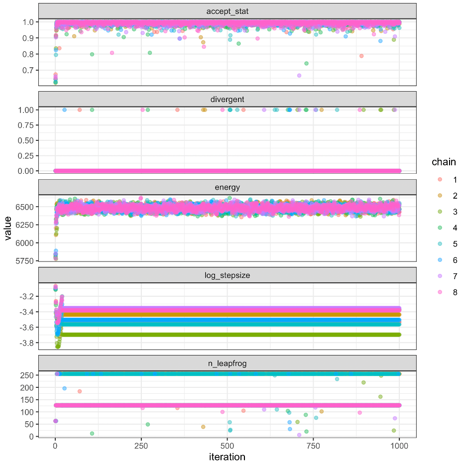
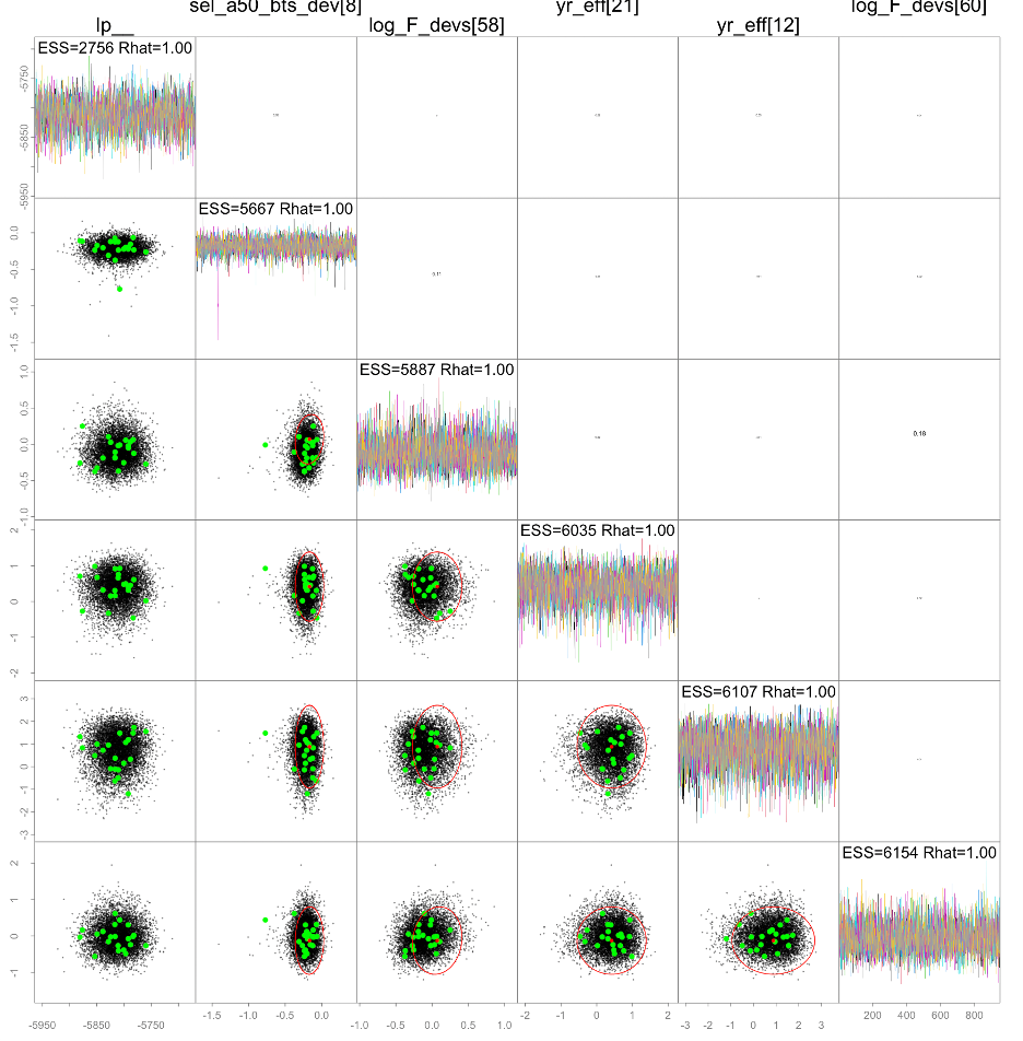
Updating the 2023 model for MCMC runs using ADNUTS, we were able to achieve reasonable statistics but some divergent transitions remained. Investigations showed that they were reasonable. Figure 32 shows some of the summary figures related to the MCMC sampling and Figure 33 shows relationships between the slowest mixing parameters. The result from sampling showed that for the 1340 parameters, there were 1,000 iterations over 8 chains with an average run time per chain of 12 minutes. The minimum effective sample size was 2,756 (36.26%) and and the maximum \(\hat{R}\) was 1.004 with 21 divergences.
Alternative software platforms
There is continued interest in using alternative software platforms for this assessment. A repository was developed for these alternatives here. The main reason for this is to provide options for upgrading the base software and providing some of the trade-offs between tailored assessments and general packages. In addition to the current model used for EBS pollock, alternaive platforms considered were:
Stock Synthesis 3: A very popular software platform
GOA pollock model: A customized program convertible between ADMB and TMB
SAM: A state-space model for age-structured assessments
AMAK: A general model assessment model developed to have flexible number of fisheries, indices etc.
WHAM: The Woods Hole Assessment Model (written in TMB…withdrawn from this presentation due to limits on time)
Each platform was intended to include as much of the configuration and baseline data from the pollock model as possible. Very little effort was made to do fine-scale bridging.
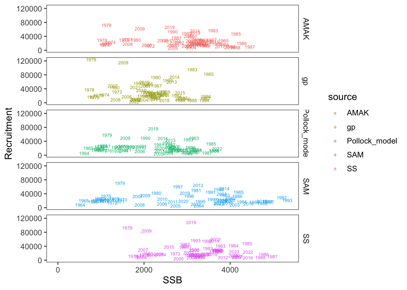
In subsequent sections we compare how the selectivity estimates compare, along with spawning biomass and recruitment.
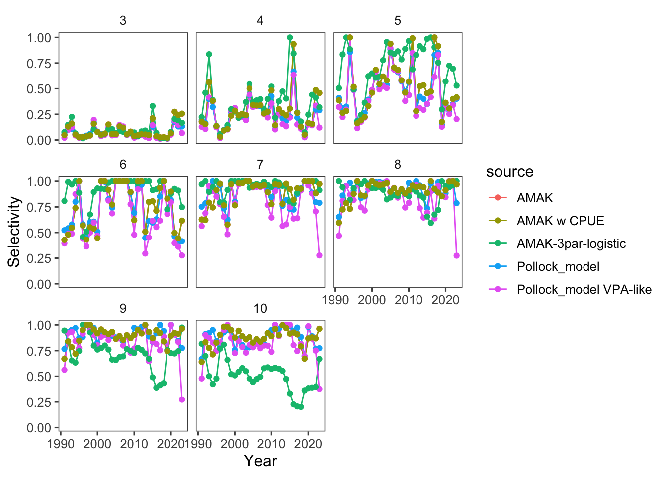
Comparing base results over different platforms
Our first pass at comparing models involved examining how selectivity could be specified and fit with the different platforms. The success in coming close to matching the pattern estimated in the present assessment varied among different platforms (Figure 34). An alternative presentation shows the differences by age over time (Figure 35). These preliminary runs over different platforms showed important differences in spawning biomass and recruits with the current assessment coming in below expectations (Figure 36). The differences for the SRR were also noteworthy (Figure 37).

Additional AMAK runs
In an attempt to get different platforms closer to each other, some tuning of the model specification for AMAK was undertaken. This included some comparisons with the early CPUE data added, and with a newly developed 3-parameter double logistic parameterization:
base: selectivity at age allowed to vary (sigma penalty=0.7)
cpue: As base but with the early CPUE data included
dbl_logistic: selectivity at age with TV selectivity parameters (3-parameter logistic)


Additional SS3 runs
Run description
Runs with different selectivity assumptions where:
- base: selectivity at age allowed to vary (sigma penalty=0.7)
- high: selectivity at age constrained (sigma penalty=0.05)
- mod: selectivity at age moderately constrained (sigma penalty=0.4)
- mix: selectivity at age moderately constrained for middle ages, high for older ages, loose for younger ages

Selectivity at age
SSB and recruitment
References
Aydin, Kerim, Sean Lucey, and Sarah Gaichas. 2024. Rpath: R Implementation of Ecopath with Ecosim. https://github.com/NOAA-EDAB/Rpath.
Carpenter, Bob, Andrew Gelman, Matthew D Hoffman, Daniel Lee, Ben Goodrich, Michael Betancourt, Marcus Brubaker, Jiqiang Guo, Peter Li, and Allen Riddell. 2017. “Stan: A Probabilistic Programming Language.” Journal of Statistical Software 76 (1).
Levine, Robert M, Alex De Robertis, Christopher Bassett, Mike Levine, and J. N Ianelli. 2024. “Acoustic observations of walleye pollock (Gadus chalcogrammus) migration across the US-Russia boundary in the northwest Bering Sea.” ICES Journal of Marine Science 81 (6): 1111–25. https://doi.org/10.1093/icesjms/fsae071.
Low, L.-L. 1983. “Application of a Laevastu-Larkins Ecosystem Model for Bering Sea Groundfish Management.” 83-02. Seattle, WA: Northwest; Alaska Fisheries Center, National Marine Fisheries Service, NOAA. https://apps-afsc.fisheries.noaa.gov/Publications/ProcRpt/PR1983-02.pdf.
Monnahan, Cole C. 2024. “Toward Good Practices for Bayesian Data-Rich Fisheries Stock Assessments Using a Modern Statistical Workflow.” Fisheries Research 275: 107024. https://doi.org/https://doi.org/10.1016/j.fishres.2024.107024.
Stock, Brian C., and Timothy J. Miller. 2021. “The Woods Hole Assessment Model (WHAM): A General State-Space Assessment Framework That Incorporates Time- and Age-Varying Processes via Random Effects and Links to Environmental Covariates.” Fisheries Research 240 (August): 105967. https://doi.org/10.1016/j.fishres.2021.105967.
Trijoulet, Vanessa, Gavin Fay, and Timothy J. Miller. 2020. “Performance of a State-Space Multispecies Model: What Are the Consequences of Ignoring Predation and Process Errors in Stock Assessments?” Journal of Applied Ecology 57 (1): 121–35. https://doi.org/https://doi.org/10.1111/1365-2664.13515.
Whitehouse, George A., and Kerim Y. Aydin. 2020. “Assessing the Sensitivity of Three Alaska Marine Food Webs to Perturbations: An Example of Ecosim Simulations Using Rpath.” Ecological Modelling 429: 109074. https://doi.org/https://doi.org/10.1016/j.ecolmodel.2020.109074.
Footnotes
This modification of Tier 2 simply applies the harmonic mean of \(F_{MSY}\) instead of the arithmetic mean to make it slightly more precautionary.↩︎