Getting Started
getting_started.RmdLoading & viewing your data
The example shown here will include a simulated spatial process giving rise to heterogeneity in fish length-at-age with a predominant north-south cline.
The first step is to ensure your data are formatted correctly and to
be aware of any sample size issues. This is accomplished via
check_data(), which returns plots of the observations and
residuals.
library(growthbreaks)
data(simulated_data) ## from the package
head(simulated_data)
#>   year age    length      lat      long
#> 2    1   1  5.174880 56.97959 -156.2602
#> 3    1   1  6.532786 57.34694 -142.2419
#> 5    1   2  9.067383 56.61224 -151.8233
#> 7    1   2 13.178737 67.63265 -169.8984
#> 8    1   2 16.415712 55.14286 -169.2174
#> 9    1   2 19.372655 51.46939 -148.3869
p <- check_data(simulated_data, showPlot = FALSE)
The first plot (p[[1]]) shows the input data, colored by
year:
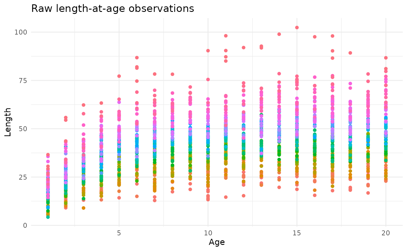
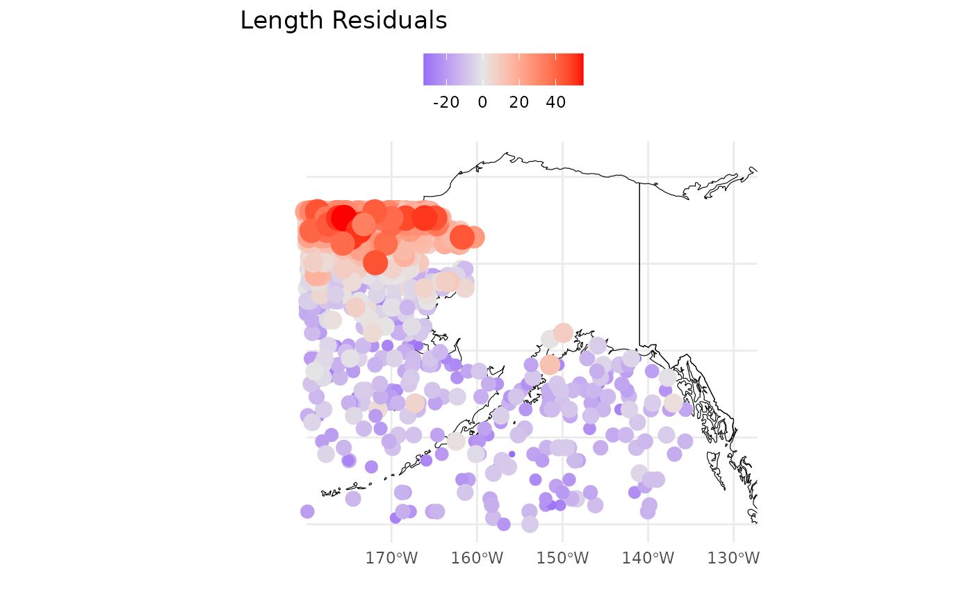
The second two plots p[[2]];p[[3]] are maps of the
observations and simple residuals (observation minus age-specific mean).
The red colors are the highest values. We’d expect these to look similar
to one another.

Once you’ve completed that step you are ready to investigate
potential breakpoints in length-at-age via get_Breaks().
This example will use the default option axes = 0 which
looks for spatial breakpoints only. The function is ignorant of any
underlying structure in the data and is not fitting growth curves at
this time. If you keep the default settings you will get back plots of
the hypothesized breaks as well as a dataframe with the breakpoints.
Detecting Breakpoints
Now we can pass our data to get_Breaks().
The ages_to_use argument allows you to specify a subset
of your age observations for which you’d like to test for breakpoints.
If you are unsure, you may choose to use age(s) that are well sampled in
your data, or all ages. However, you will want to include at least some
observations of small (young) fish, since discrepancies in size may be
less obvious for fish at or near their asymptotic length. Here I am
testing three ages and saving the output to a dataframe called
breakpoints.
breakpoints <- get_Breaks(dat = simulated_data,
                          ages_to_use = c(5,10,15),
                          sex = FALSE,
                          axes = 0,
                          showPlot = FALSE)
breakpoints$breakpoints
#>         lat      long detected_break      freq
#> 87 65.63636 -141.4534           TRUE 0.3333333
plot_Breaks(dat=simulated_data, breakpoints$breakpoints, showData =  TRUE)
As we might have expected based on the raw observations, the algorithm
detected a break at about
N,
as well as an unexpected one at
W.
We can see this on the map as well as in the dataframe. The
As we might have expected based on the raw observations, the algorithm
detected a break at about
N,
as well as an unexpected one at
W.
We can see this on the map as well as in the dataframe. The
count column indicates the proportion of tested ages for
which this breakpoint was detected (in this case, 1/3, suggesting that
no breakpoints were detected for 2/3 ages). You may choose to stop
here. If you’re interested in some of the automated checking and curve
fitting functionality, proceed to the next step.
Re-fitting growth curves at putative breaks
The function refit_Growth() can be used to generate
plots of the growth parameters and associated curves by splitting your
data into the spatio/temporal zones (“strata”) defined by
breakpoints. This can allow you to make inferences about a)
the magnitude and significance of differences in individual parameters
and b) the resultant impact on our perception of length-at-age.
It is common for growth curves to be very similar especially when the number of strata is large (>3), so user judgment is required to discern the best use of the information provided here.
Run the function with the breakpoints as-is and inspect the outputs.
fits1 <- refit_Growth(simulated_data, breakpoints$breakpoints, showPlot = FALSE)

names(fits1$split_tables) ## description of the strata used
#> [1] "lat_less_66_long_less_-141"    "lat_greater_66_long_less_-141"
#> [3] "lat_less_66_long_greater_-141"
## split_tables contains your observed data broken up by strata
We can inspect the fitted curves in two ways: first, by visualizing
the $par_plot. The red points & error bars indicate
estimates for which the mean fell outside the confidence interval(s) for
other strata. This can be used to infer which components of the growth
curve are possibly contributing to detected differences among strata. It
doesn’t look like the second strata’s
nor
values are very different than the other regions’.
The AIC of this first model is given by fits1$AIC:
1.4499293^{4}.
fits1$pars_plot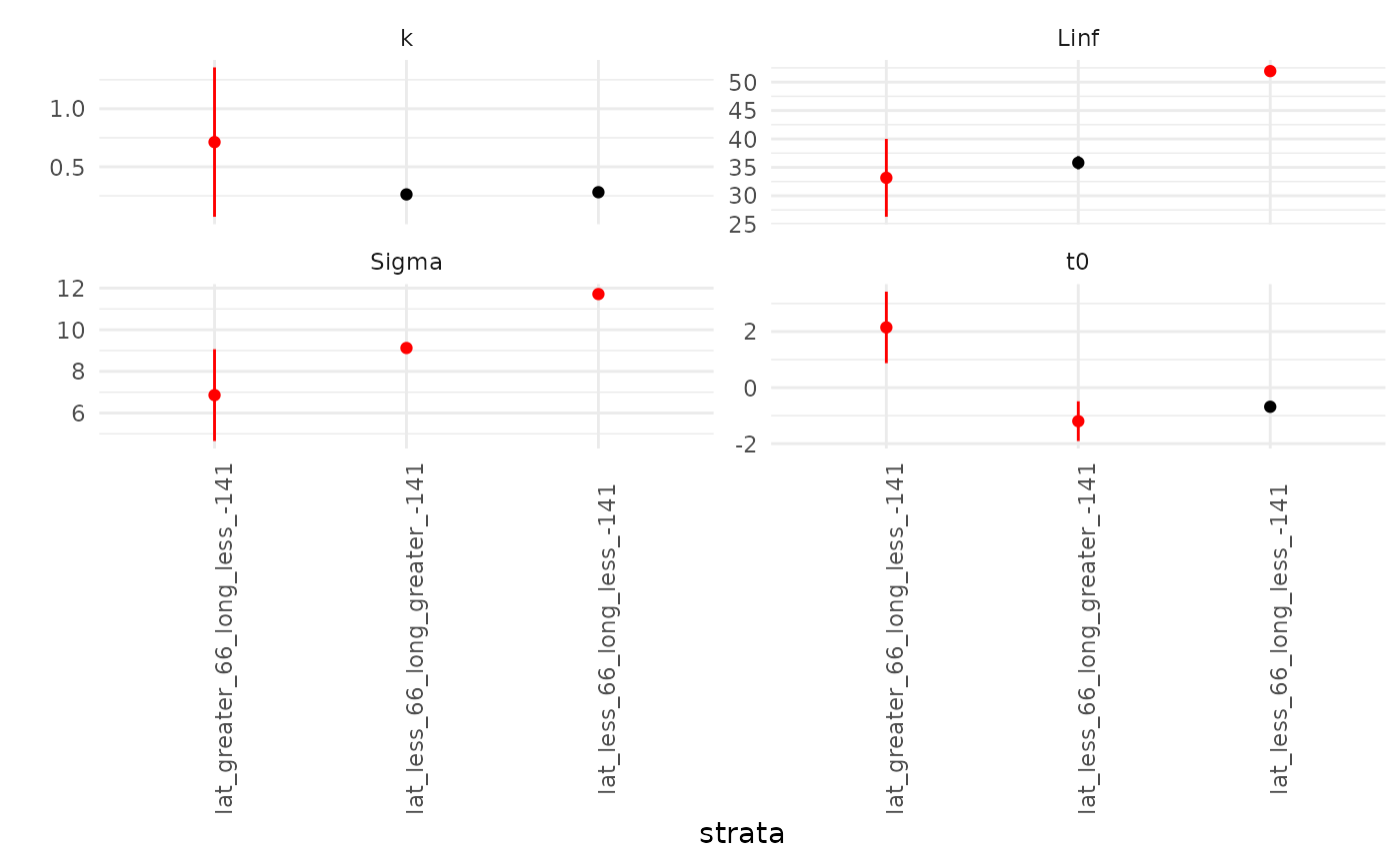
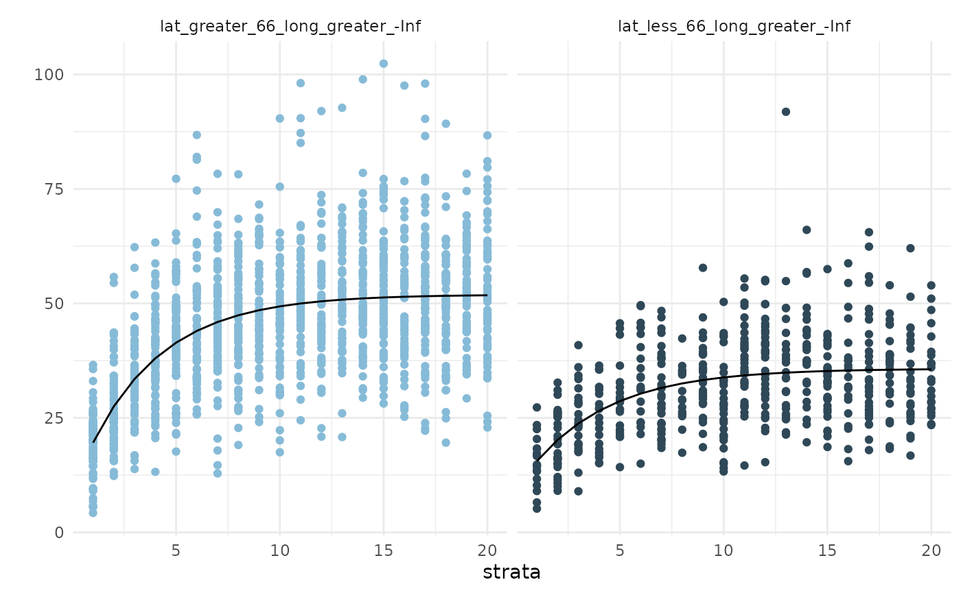
The second way to explore the results are by visualizing the fitted
curves against the strata-specific observations contained in
$fits_plot. Here we see that the second and third strata
(all data points below
)N
exhhibit very similar curves, and there are not many data points in the
second strata to begin with.
fits1$fits_plot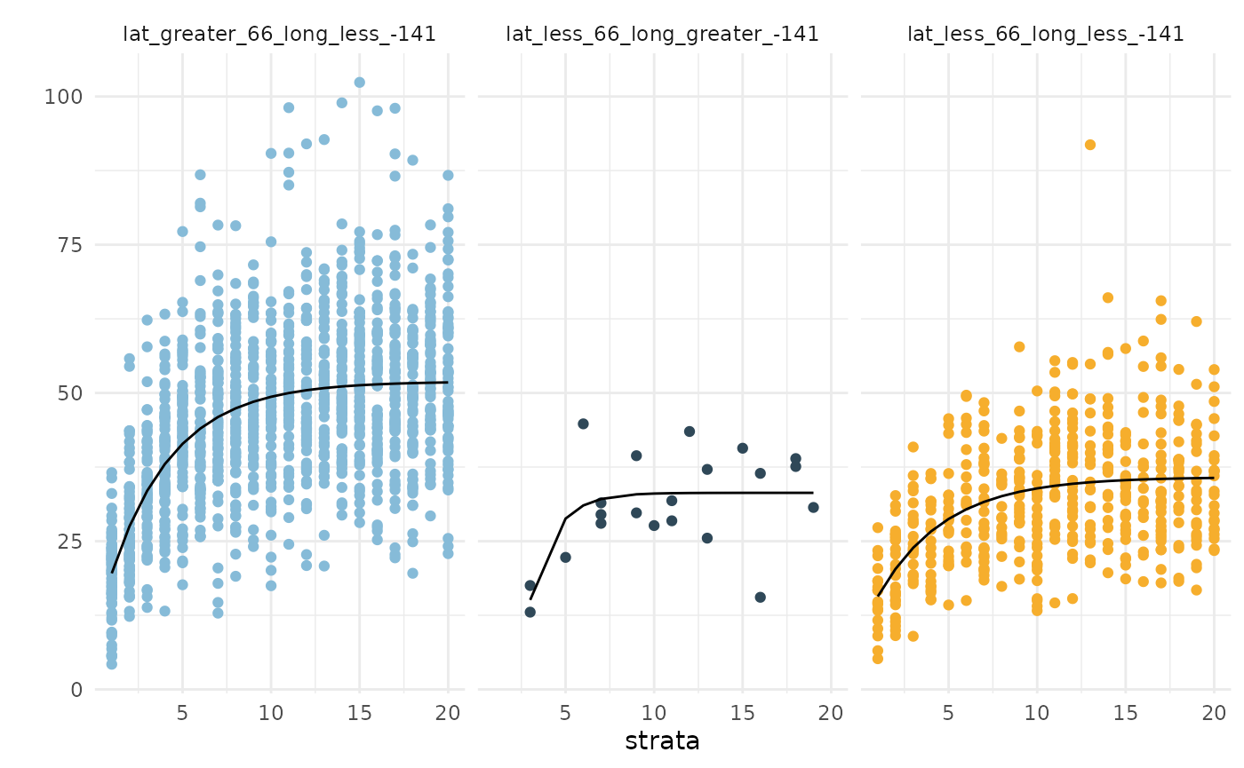
Updating and re-fitting the breakpoints
Based on the exploration above, you may decide to manually combine
the second and third strata, using just a single breakpoint north to
south. In this case, we would do away with the breakpoint at
)W,
replacing it with -Inf.
breakpoints$breakpoints$long <- -Inf
fits2 <- refit_Growth(simulated_data,
                      breakpoints$breakpoints,
                      showPlot = FALSE) ## refit the curves
We can repeat the visualization and see that 1) the key parameter
values are now more distinct from one another and 2) so are the
curves.The AIC of this updated model is given by fits2$AIC:
1.4496484^{4}, for a
AIC
of 2.8091856.
fits2$pars_plot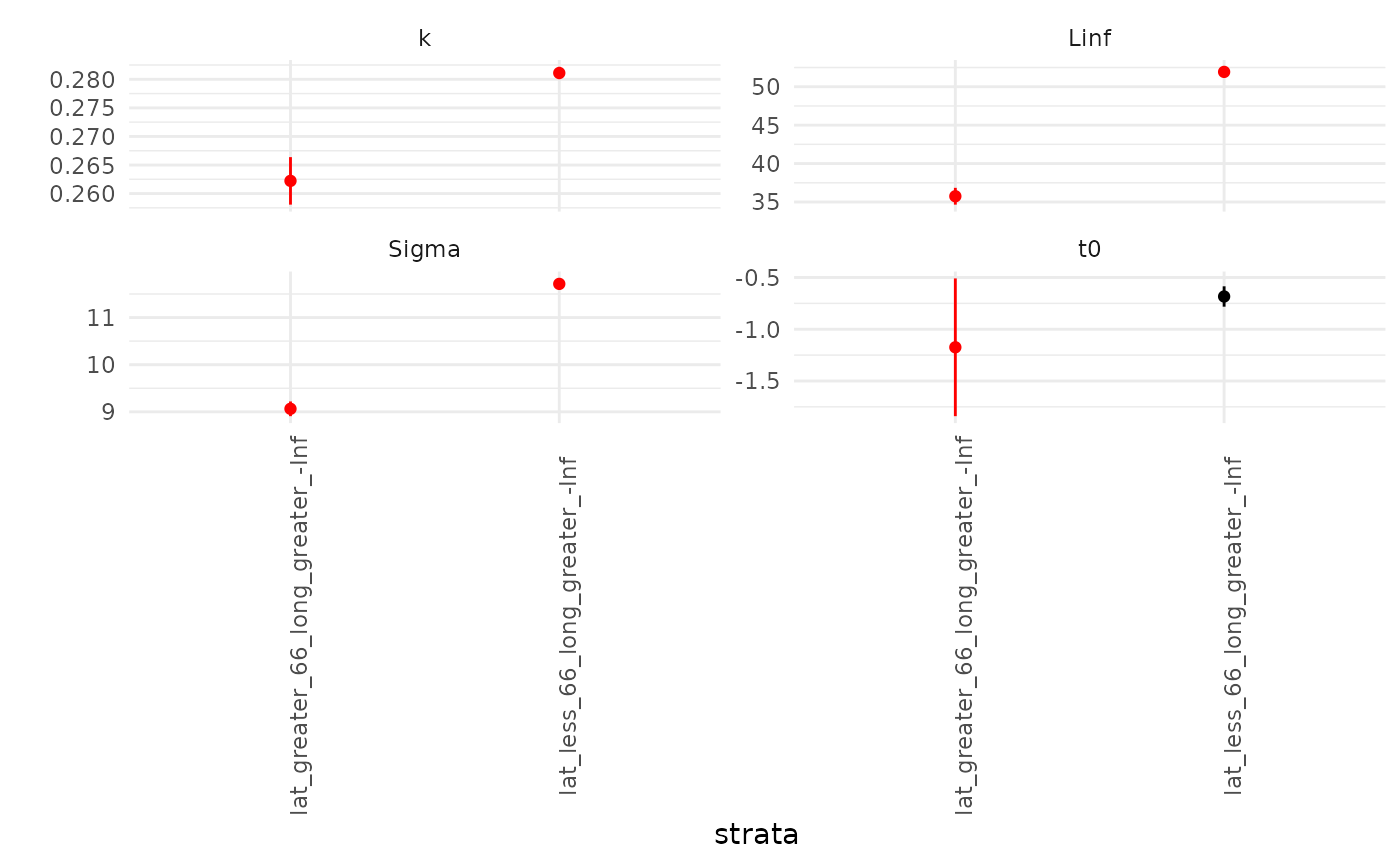
fits2$fits_plot