REMA basics

library(rema)
library(ggplot2)
library(dplyr)
library(knitr)

ggplot2::theme_set(cowplot::theme_cowplot(font_size = 14) +
                     cowplot::background_grid() +
                     cowplot::panel_border())

In this series of vignettes we walk through several examples of how to prepare and fit a suite of random effects (RE) models for biomass estimation and apportionment using the rema package.

The rema workflow:

1. Load rema and data. The user can read biomass or other abundance index data from file (e.g. .csv file), or they can use the rwout.rep report file from the ADMB version of the RE model using read_admb_re().

2. Specify model structure and assumptions using prepare_rema_input(). This function allows users to quickly transition from a single to two survey model, specify alternative process error structures, add likelihood penalties or priors on parameters, and evaluate alternative assumptions about zero biomass observations.

3. Fit the specified REMA model using fit_rema() and determine whether the model has met basic convergence criteria (e.g., Hessian is positive definite, a maximum gradient component approximately equal to zero).

4. Extract rema model output into clean, consistently formatted data frames using tidy_rema(). The user can visualize this model output using plot_rema(), or quickly format it into tables for a report.

5. Compare alternative REMA models and conduct model selection using compare_rema_models(). Output from this function includes a table of Akaike Information Criteria (AIC) when appropriate, figures, and tidied data frames. This function also accepts model output from the ADMB version of the RE model for easy comparison to past models.

Taken together, these functions allow R users to quickly fit and interrogate a suite of simple statistical models in TMB without needing software-specific training or expertise.

Example 1: Univariate random effects (RE) model with a single survey and stratum

This example uses Aleutian Islands shortraker (aisr_rwout.rep) and fits to NMFS bottom trawl survey estimates.

1. Read in the rwout.rep, a custom report file generated by the ADMB version of the random effects model.

# ?read_admb_re
admb_re <- read_admb_re(filename = 'aisr_rwout.rep',
                        # optional label for the single biomass survey stratum
                        biomass_strata_names = 'Aleutians Islands',
                        model_name = 'ADMB: AI shortraker')
names(admb_re)
#> [1] "biomass_dat"           "cpue_dat"              "model_yrs"            
#> [4] "init_log_biomass_pred" "admb_re_results"
kable(admb_re$biomass_dat)

strata	year	biomass	cv
Aleutians Islands	1980	6829.3	0.5531111
Aleutians Islands	1983	26275.5	0.2006878
Aleutians Islands	1986	11667.2	0.2505718
Aleutians Islands	1991	21835.4	0.6916255
Aleutians Islands	1994	26284.4	0.2198947
Aleutians Islands	1997	36058.3	0.2694324
Aleutians Islands	2000	37151.8	0.4460828
Aleutians Islands	2002	15342.0	0.2009741
Aleutians Islands	2004	32611.6	0.3743298
Aleutians Islands	2006	11780.6	0.2522081
Aleutians Islands	2010	18223.7	0.2336468
Aleutians Islands	2012	15667.7	0.2636677
Aleutians Islands	2014	16400.5	0.3771796
Aleutians Islands	2016	15024.0	0.3199997

2. Prepare REMA model inputs using the admb_re data object.

# ?prepare_rema_input 
input <- prepare_rema_input(model_name = 'TMB: AI shortraker', admb_re = admb_re)
names(input) 
#> [1] "data"        "par"         "map"         "random"      "model_name" 
#> [6] "osa"         "biomass_dat"

The input$data, input$par, input$map, and input$random are used by TMB to fit the REMA model. The other objects are used by other functions to process model results or conduct residual analyses.

Data could alternatively be entered into prepare_rema_input() using the biomass_dat argument:

# (not run)
input <- prepare_rema_input(model_name = 'tmb_rema_aisr', biomass_dat = admb_re$biomass_dat)

3. Fit REMA model

# ?fit_rema
m <- fit_rema(input)
#> Model runtime: 0.1 seconds 
#> stats::nlminb thinks the model has converged: mod$opt$convergence == 0
#> Maximum gradient component: 1.90e-11 
#> Max gradient parameter: log_PE 
#> TMB:sdreport() was performed successfully for this model

4. Get tidied model output and plot results

Note that the 95% confidence intervals of the observations (i.e., obs_lci and obs_uci in output$biomass_by_strata are based on the assumption of normality in log-space; therefore, they are asymmetric on the arithmetic scale.

# ?tidy_rema
output <- tidy_rema(rema_model = m)
kable(output$parameter_estimates) # estimated fixed effects parameters

model_name	parameter	estimate	std_err	lci	uci
TMB: AI shortraker	process_error	0.1557776	0.1044475	0.0418584	0.5797328

kable(head(output$biomass_by_strata, 5)) # data.frame of predicted and observed biomass by stratum

model_name	strata	variable	year	log_pred	sd_log_pred	pred	pred_lci	pred_uci	obs	obs_cv	log_obs	sd_log_obs	obs_lci	obs_uci
TMB: AI shortraker	Aleutians Islands	biomass_pred	1980	9.689900	0.3344752	16153.63	8386.182	31115.44	6829.3	0.5531111	8.828978	0.51664	2480.912	18799.27
TMB: AI shortraker	Aleutians Islands	biomass_pred	1981	9.768171	0.2704639	17468.78	10281.186	29681.23	NA	NA	NA	NA	NA	NA
TMB: AI shortraker	Aleutians Islands	biomass_pred	1982	9.846441	0.2155808	18891.00	12380.902	28824.23	NA	NA	NA	NA	NA	NA
TMB: AI shortraker	Aleutians Islands	biomass_pred	1983	9.924711	0.1784564	20429.01	14399.421	28983.43	26275.5	0.2006878	10.176392	0.19871	17799.538	38787.63
TMB: AI shortraker	Aleutians Islands	biomass_pred	1984	9.848307	0.1919367	18926.28	12992.373	27570.34	NA	NA	NA	NA	NA	NA

# ?plot_rema
plots <- plot_rema(tidy_rema = output, biomass_ylab = 'Biomass (t)') # optional y-axis label
plots$biomass_by_strata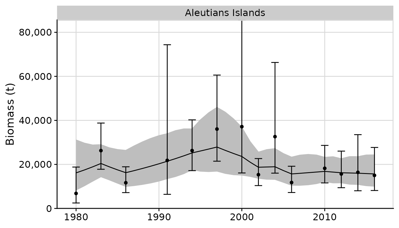

5. Compare with ADMB RE model results

# ?compare_rema_models
compare <- compare_rema_models(rema_models = list(m),
                               admb_re = admb_re,
                               biomass_ylab = 'Biomass (t)')
compare$plots$biomass_by_strata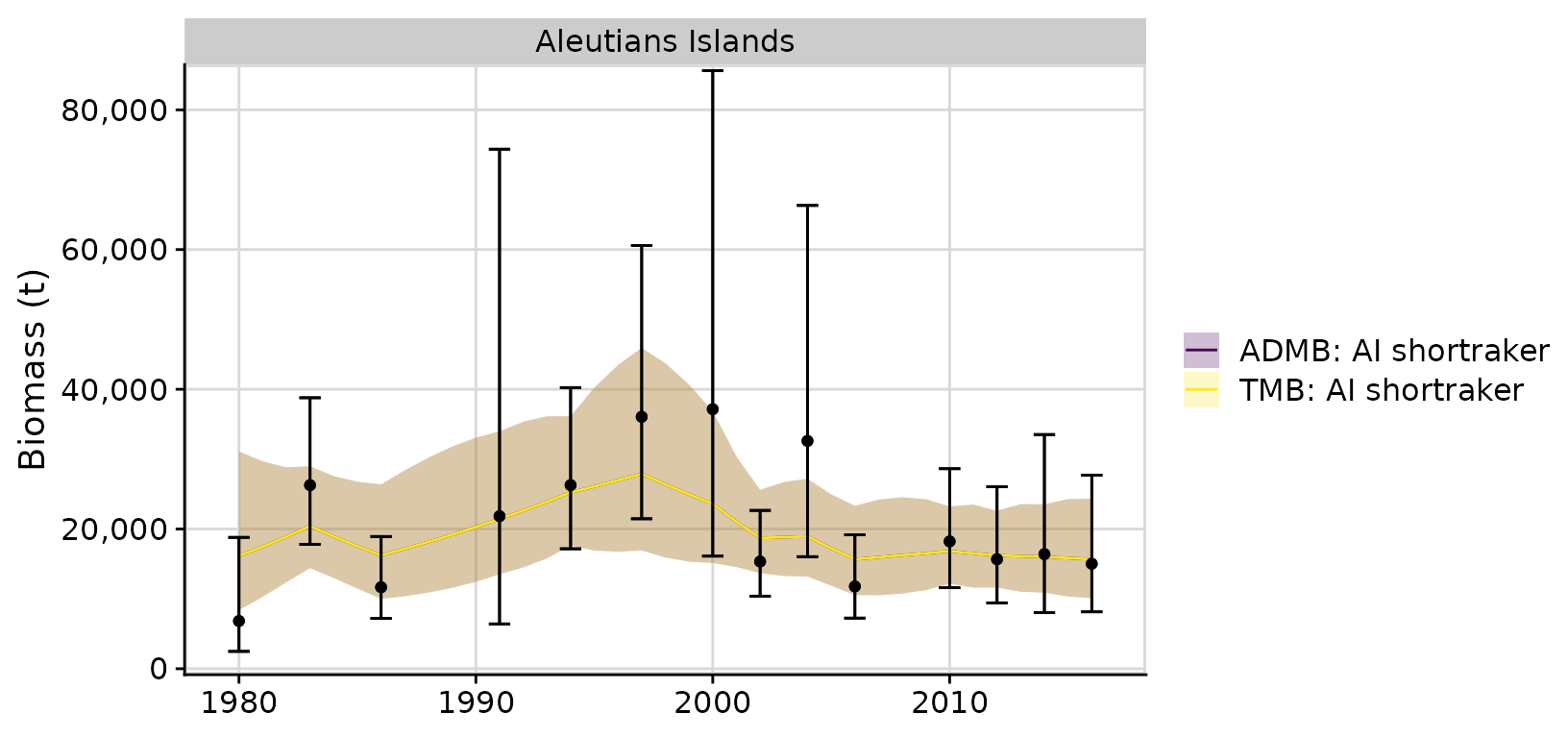

Example 2: Multivariate random effects model (REM) with a single survey and multiple strata

This example uses Bering Sea and Aleutian Islands shortspine thornyhead (bsaisst_rwout.rep) and fits to the NMFS EBS slope and AI bottom trawl survey estimates. The original ADMB model has a single, shared process error (PE) over the three strata. This example demonstrates how to define alternative PE structures, and how to u to perform model selection using AIC.

admb_re <- read_admb_re(filename = 'bsaisst_rwout.rep',
                      biomass_strata_names = c('AI survey', 'EBS slope survey', 'S. Bering Sea (AI survey)'),
                      model_name = 'ADMB: single PE')

# the original ADMB model shared PE across all strata
input1 <- prepare_rema_input(model_name = 'TMB: single PE',
                            admb_re = admb_re,
                            PE_options = list(pointer_PE_biomass = c(1, 1, 1)))
m1 <- fit_rema(input1)
#> Model runtime: 0.1 seconds 
#> stats::nlminb thinks the model has converged: mod$opt$convergence == 0
#> Maximum gradient component: 9.81e-10 
#> Max gradient parameter: log_PE 
#> TMB:sdreport() was performed successfully for this model
output <- tidy_rema(rema_model = m1)
kable(output$parameter_estimates) # estimated fixed effects parameters

model_name	parameter	estimate	std_err	lci	uci
TMB: single PE	process_error	0.121168	0.0286548	0.0762236	0.1926136

kable(head(output$biomass_by_strata, 5)) # data.frame of predicted and observed biomass by stratum

model_name	strata	variable	year	log_pred	sd_log_pred	pred	pred_lci	pred_uci	obs	obs_cv	log_obs	sd_log_obs	obs_lci	obs_uci
TMB: single PE	AI survey	biomass_pred	1982	8.792938	0.4034013	6587.561	2987.781	14524.48	NA	9.000024	NA	NA	NA	NA
TMB: single PE	AI survey	biomass_pred	1983	8.792938	0.3847739	6587.561	3098.878	14003.76	NA	9.000024	NA	NA	NA	NA
TMB: single PE	AI survey	biomass_pred	1984	8.792938	0.3651976	6587.561	3220.089	13476.63	NA	9.000024	NA	NA	NA	NA
TMB: single PE	AI survey	biomass_pred	1985	8.792938	0.3445106	6587.561	3353.333	12941.14	NA	9.000024	NA	NA	NA	NA
TMB: single PE	AI survey	biomass_pred	1986	8.792938	0.3224994	6587.560	3501.165	12394.72	NA	9.000024	NA	NA	NA	NA

kable(head(output$total_predicted_biomass, 5)) # combined/total predicted biomass

model_name	variable	year	pred	pred_lci	pred_uci
TMB: single PE	tot_biomass_pred	1982	24821.5	11212.94	54946.07
TMB: single PE	tot_biomass_pred	1983	24821.5	11446.45	53825.14
TMB: single PE	tot_biomass_pred	1984	24821.5	11691.42	52697.34
TMB: single PE	tot_biomass_pred	1985	24821.5	11948.96	51561.54
TMB: single PE	tot_biomass_pred	1986	24821.5	12220.35	50416.45

We can use ggplot2 functions to modify formatting of plots:

plots <- plot_rema(tidy_rema = output, biomass_ylab = 'Biomass (t)')
plots$biomass_by_strata + facet_wrap(~strata, ncol = 1, scales = 'free_y')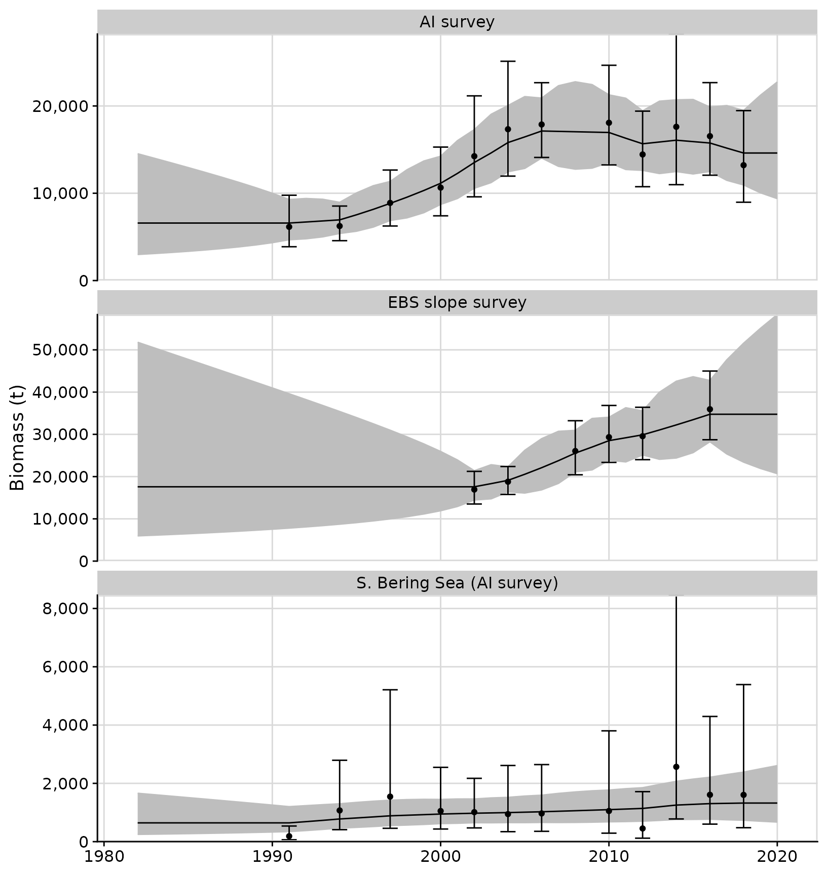

One of the primary uses for the RE model is apportioning catch by management area. The tidy_rema() function output includes a table with proportions of predicted biomass by strata:

kable(tail(output$proportion_biomass_by_strata, 3)) 

model_name	year	AI survey	EBS slope survey	S. Bering Sea (AI survey)
TMB: single PE	2018	0.2882088	0.6856694	0.0261218
TMB: single PE	2019	0.2882088	0.6856694	0.0261218
TMB: single PE	2020	0.2882088	0.6856694	0.0261218

# figure:
# plots$proportion_biomass_by_strata

We can compare the TMB model results with the original ADMB model. Note different confidence intervals in the ADMB and TMB versions. The ADMB code uses the Marlow method to sum the variances of biomass in log-space, whereas the TMB version applies the standard Delta method.

compare <- compare_rema_models(rema_models = list(m1),
                               admb_re = admb_re,
                               biomass_ylab = 'Biomass (t)')

# Note different confidence intervals between the ADMB version (Marlow method) and the TMB version (Delta method)
compare$plots$biomass_by_strata + facet_wrap(~strata, ncol = 1, scales = 'free_y')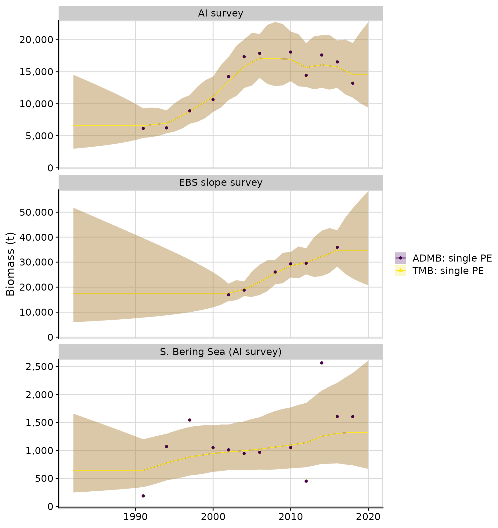

compare$plots$total_predicted_biomass + ggplot2::ggtitle('BSAI Shortspine thornyhead')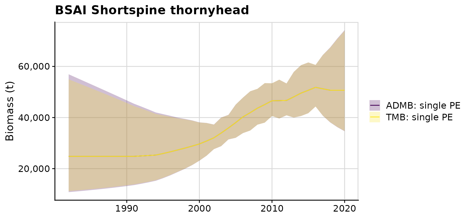 

We can easily fit an alternative REMA model with strata-specific PE parameters, and compare the two models using AIC. In this case we see the single PE model has the lowest AIC value. Note that ADMB models cannot currently be compared with REMA models using AIC, therefore we omit the admb_re = admb_re argument in the compare_rema_models() function call below:

# REMA defaults to strata-specific parameters, which could be explicitly defined
# as: PE_options = list(pointer_PE_biomass = c(1, 2, 3))
input2 <- prepare_rema_input(model_name = 'TMB: strata-specific PE',
                            admb_re = admb_re) 

m2 <- fit_rema(input2)
#> Model runtime: 0.3 seconds 
#> stats::nlminb thinks the model has converged: mod$opt$convergence == 0
#> Maximum gradient component: 2.31e-07 
#> Max gradient parameter: log_PE 
#> TMB:sdreport() was performed successfully for this model

compare <- compare_rema_models(rema_models = list(m1, m2),
                               biomass_ylab = 'Biomass (t)')

compare$plots$biomass_by_strata + facet_wrap(~strata, ncol = 1, scales = 'free_y')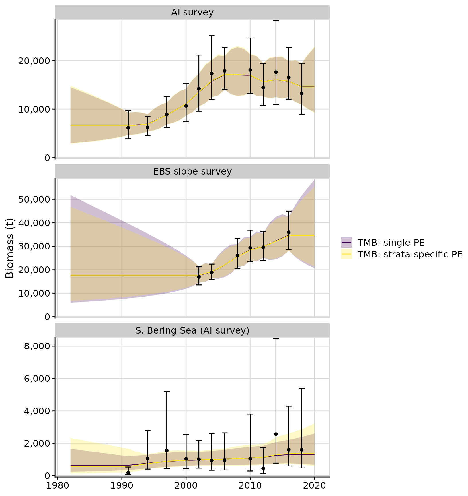

kable(compare$aic)

model_name	objective_function	n_parameters	aic	delta_aic
TMB: single PE	34.73785	1	71.5	0.0
TMB: strata-specific PE	34.65104	3	75.3	3.8

kable(compare$output$parameter_estimates)

model_name	parameter	estimate	std_err	lci	uci
TMB: single PE	process_error	0.1211680	0.0286548	0.0762236	0.1926136
TMB: strata-specific PE	process_error	0.1257423	0.0384807	0.0690223	0.2290726
TMB: strata-specific PE	process_error	0.1084952	0.0419428	0.0508566	0.2314587
TMB: strata-specific PE	process_error	0.1552381	0.1289141	0.0304885	0.7904241