REMA model validation

Background

Fisheries stock assessments are moving towards state-space estimation, which boasts a range of benefits, including separation and estimation of observation and process error, a more elegant framework for handling missing data, a high degree of flexibility with respect to model architecture and inclusion of different data types, and the potential for improved projections and predictive skill (Aeberhard et al., 2018). The flexibility and relative ease of fitting state-space models means they can increase in complexity and dimensionality rapidly. While easy to fit, state-space models are often challenging to validate, and even simple models can suffer from estimation issues that result in biased inference (Auger‐Méthé et al., 2016).

At the North Pacific Fishery Management Council (NPFMC), the “random effects model” (REMA) is by far the most common state-space model used for fishery management (Sullivan et al., 2022). REMA is a state-space random walk model that can be customized to estimate multiple process errors, fit to an additional abundance index, or estimate additional observation error. REMA is used to estimate biomass within Tier 5 groundfish and Tier 4 crab stock assessments and to apportion Acceptable Biological Catches (ABCs) by management area for many stocks. Despite the high impact of this model within the North Pacific fishery management process, we have no standard model validation practices for REMA.

Our goals:

Apply established state-space model validation techniques to real life REMA examples.
Create a REMA model validation guide with clear descriptions of each method and motivation for its use, an explanation of how to interpret the model validation results, and reproducible code that will run for all operational REMA models at the NPFMC.
Provide preliminary recommendations for REMA users and reviewers on which model validation methods are most relevant and informative for REMA.

Interested but otherwise busy readers are encouraged to skip to the “When should we care about failed model diagnostics?” and “Recommendations” sections. Table 1 and Figures 6-8 show examples of a REMA model failing model validation criteria.

A testing framework for REMA model validation

In this analysis, we will be testing that (1) REMA is working as expected (i.e., code has been implemented correctly and parameters are estimated without bias), and (2) that the assumptions made when parameterizing and estimating REMA are valid, including assumptions related to random effects and error structure. We use two example stocks:

Aleutian Islands Pacific cod (AI Pcod; Spies et al., 2023): a simple, univariate case, which fits to a single time series of the AI bottom trawl survey and estimates one process error
Gulf of Alaska Thornyhead rockfish (GOA thornyhead; Echave et al., 2022): a complex, multi-strata and multi-survey case, which estimates multiple process errors, a scaling parameter for the longline survey, and two additional observation errors for the GOA bottom trawl and longline surveys

Both models appear to converge per standard REMA and TMB diagnostics (small maximum gradient, invertible Hessian), and fit the data reasonably, with model fits shown in Figure 1. These stocks span the levels of complexity of NPFMC REMA models; testing REMA across this range of complexity helps ensure that model and model assumptions are valid in a variety of realistic, management-relevant cases.

It is important to note that model validation does not mean the model is “more right” or “more correct.” Model validation does not help an analyst with model selection (except to identify models that might not function properly), nor does it ensure that the model makes “better” predictions. Rather, model validation is a way to ensure that the model is operating as expected, without introducing bias or violating statistical assumptions upon which the model is based (Auger‐Méthé et al., 2016; Auger‐Méthé et al., 2021), and that the data reasonably could have come from the model (Thygesen et al., 2017).

The key questions we aim to answer with model validation include the following:

Does the model perform as expected, or does it introduce bias? Using a simulation self-check, we will test if the model is coded correctly and is able to recover known parameters.
Is it plausible that our data could have been generated by the model? Using one-step ahead (OSA) residuals, the appropriate residual type for state-space models, we test the model assumptions and look for trends in residuals that reveal characteristics or dynamics of the data that aren’t adequately captured by the model.
Are the normality assumptions made when estimating random effects via the Laplace approximation accurate? By comparing the posterior distribution of fixed effects with and without the Laplace approximation, we test whether the distribution of the random effects are normal and thus the accuracy of the Laplace approximation. This allows us to test the accuracy of the fixed effects estimates with uncertainties.
Are the parameters unique and non-redundant? Checking the correlation between parameters helps us identify if parameters are redundant with each other.

Prepare data for each stock here

First, we run the model for each stock. The AI Pcod model (pcod_mod) uses a single process error to describe the stock over time (one parameter). The GOA thornyhead rockfish model (thrn_mod) uses data from two surveys (bottom trawl and longline survey) to describe the stock over time (six fixed effects parameters: three process errors, one scaling parameter, additional observation error for the biomass survey, and additional observation error for the longline survey).

In the code below, we show how to specify and fit these models within the rema framework and plot fits to the data. Figure 1 shows the fits to the data for AI Pcod and GOA Thornyhead. In particular, the GOA Thornyhead fits show a trade off between the biomass and longline survey data.


set.seed(415) # for reproducibility, use a seed

# first, get the p-cod data set up
pcod_bio_dat <- read.csv("ai_pcod_2022_biomass_dat.csv")
pcod_input <- prepare_rema_input(model_name = "p_cod",
                                 biomass_dat = pcod_bio_dat,
                                 # one strata
                                 PE_options = list(pointer_PE_biomass = 1)
                                 )
# run the model
pcod_mod <- fit_rema(pcod_input) 

# next, get the thornyhead data set up
thrn_bio_dat <- read.csv("goa_thornyhead_2022_biomass_dat.csv")
thrn_cpue_dat <-read.csv("goa_thornyhead_2022_cpue_dat.csv")
thrn_input <- prepare_rema_input(model_name = 'thrnhead_rockfish',
                                multi_survey = TRUE,
                                biomass_dat = thrn_bio_dat,
                                cpue_dat = thrn_cpue_dat,
                                # RPWs are a summable/area-weighted effort index
                                sum_cpue_index = TRUE, 
                                # three process error parameters (log_PE) estimated,
                                # indexed as follows for each biomass survey stratum
                                # (shared within an area across depths):
                                PE_options = list(pointer_PE_biomass = c(1, 1, 1, 2, 2, 2, 3, 3, 3)),
                                # scaling parameter options:
                                q_options = list(
                                # longline survey strata (n=3) indexed as follows for the
                                # biomass strata (n=9)
                                pointer_biomass_cpue_strata = c(1, 1, 1, 2, 2, 2, 3, 3, 3),
                                # one scaling parameters (log_q) estimated, shared
                                # over all three LLS strata
                                pointer_q_cpue = c(1, 1, 1)),
                                # estimate extra trawl survey observation error
                                extra_biomass_cv = list(assumption = 'extra_cv'),
                                # estimate extra longline survey observation error
                                extra_cpue_cv = list(assumption = 'extra_cv')
                                )

# run the model
thrn_mod <- fit_rema(thrn_input) 

# tidy output and plot fitted data
tidy_pcod <- tidy_rema(pcod_mod)
p1 <- plot_rema(tidy_pcod)$biomass_by_strata + 
  ggtitle(label = "Model Fits to the AI Pcod Data",
          subtitle = "Trawl Survey Biomass Strata") + 
  geom_ribbon(aes(ymin = pred_lci, ymax = pred_uci),
              col = 'goldenrod', fill = 'goldenrod', alpha = 0.4) +
  geom_line() +
  geom_point(aes(x = year, y = obs)) +
  geom_errorbar(aes(x = year, ymin = obs_lci, ymax = obs_uci))
p1
ggsave(paste0("vignettes/ex4_pcod_fits.png"), width = 6, height = 4, units = "in", bg = "white")

tidy_thrn <- tidy_rema(thrn_mod)
p2 <- plot_rema(tidy_thrn, biomass_ylab = 'Biomass (t)')$biomass_by_strata + 
  ggtitle(label = "Model Fits to the GOA Thornyhead Data",
          subtitle = "Trawl Survey Biomass Strata") + 
  geom_ribbon(aes(ymin = pred_lci, ymax = pred_uci),
              col = "#21918c", fill = "#21918c", alpha = 0.4) +
  geom_line() +
  geom_point(aes(x = year, y = obs)) +
  geom_errorbar(aes(x = year, ymin = obs_lci, ymax = obs_uci))
p2
p3 <- plot_rema(tidy_thrn, cpue_ylab = "RPW")$cpue_by_strata + 
  ggtitle(label = NULL, subtitle = "Longline Survey Relative Population Weight (RPW) Strata") + 
  geom_ribbon(aes(ymin = pred_lci, ymax = pred_uci),
              col = "#21918c", fill = "#21918c", alpha = 0.4) +
  geom_line() +
  geom_point(aes(x = year, y = obs)) +
  geom_errorbar(aes(x = year, ymin = obs_lci, ymax = obs_uci))
p3
cowplot::plot_grid(p2, p3, rel_heights = c(0.7, 0.3), ncol = 1)
ggsave(paste0("vignettes/ex4_thrn_fits.png"), width = 11, height = 10, units = "in", bg = "white")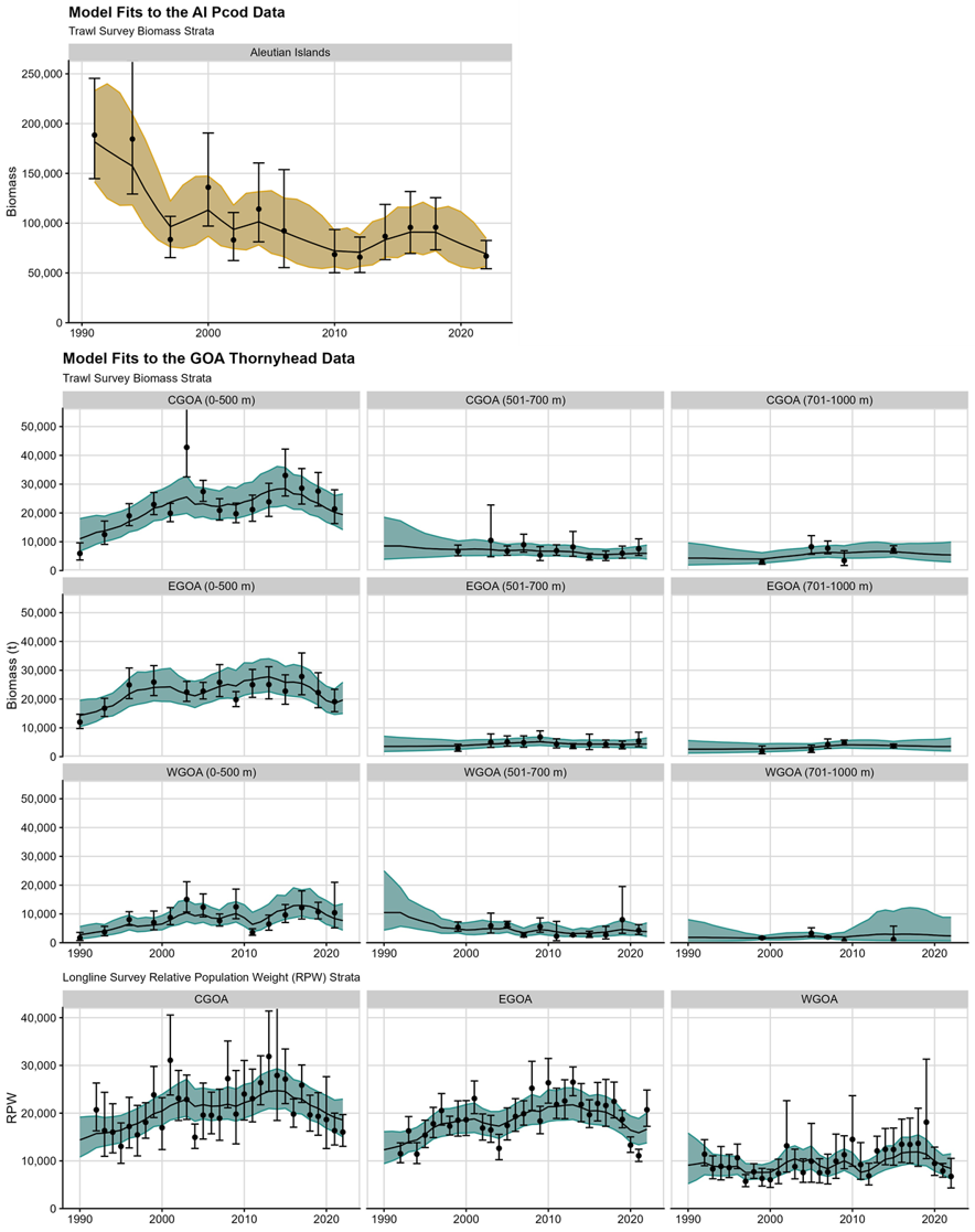

Figure 1. Fits to the AI Pcod (top panel; gold) and GOA Thornyhead (bottom panels; teal) models.

1. Simulation self-test: Can we recover parameters without bias?

Simulation testing ensures the model has been properly coded and performs consistently without introducing bias (Auger‐Méthé et al., 2021; Gimenez et al., 2004). First, we use the REMA model to estimate parameters (e.g., process error variance) from the real data. Next, we use the estimated parameters as “true values” to simulate new latent states (random effects) and data conditioned on the states using the REMA equations. We then use the REMA model to re-estimate the model parameters (“recovered parameters”) and calculate the relative error (RE; i.e., (true-estimated values)/true value*100)) for the parameters in each simulation replicate (N=500). The AI Pcod model is fitted to bottom trawl data and each simulated data set is a biomass trajectory; the GOA Thornyhead model is fitted to bottom trawl and longline survey data, and each simulation data set includes biomass trajectories in nine strata and longline survey relative population weights (RPWs) in three strata.

Models fail this simulation testing when the recovered parameters are biased (RE ≠ 0), or deviate consistently from the true values used to simulate data (span of the recovered parameters is large): this can indicate that the model has a coding error, is non-identifiable, has redundant parameters, or is biased (i.e., there is some other kind of model misspecification).

The following function runs a simulation self-test for a REMA model.


sim_test <- function(mod_name, replicates, cpue) {

  # storage things
  re_est <- matrix(NA, replicates, length(mod_name$par)) # parameter estimates

  # go through the model
  suppressMessages(for(i in 1:replicates) {

    sim <- mod_name$simulate(complete = TRUE) # simulates the data

    # simulated biomass observations:
    tmp_biomass <- matrix(data = exp(sim$log_biomass_obs), ncol = ncol(mod_name$input$data$biomass_obs))
    colnames(tmp_biomass) <- colnames(mod_name$data$biomass_obs)
    # simulated cpue observations, when applicable:
    if (cpue) {tmp_cpue <- matrix(data = sim$cpue_obs, ncol = ncol(mod_name$input$data$cpue_obs))
    colnames(tmp_cpue) <- colnames(mod_name$data$cpue_obs)}
    # set up new data for input
    newinput <- mod_name$input
    newinput$data$biomass_obs <- tmp_biomass # biomass data
    if (cpue) {newinput$data$cpue_obs <- tmp_cpue} # cpue data

    # create "obsvec" which is used internally in cpp file as the observation
    # vector for all observation (log biomass + cpue) in the likelihood
    # functions (and required for OSA residuals). note the transpose t() needed
    # to get these matrices in the correct order (by row instead of by col) --
    # note obsvec is masked from users normally in prepare_rema_input()
    newinput$data$obsvec <- t(sim$log_biomass_obs)[!is.na(t(sim$log_biomass_obs))]
    if (cpue) {newinput$data$obsvec <- c(t(sim$log_biomass_obs)[!is.na(t(sim$log_biomass_obs))], t(sim$log_cpue_obs)[!is.na(t(sim$log_cpue_obs))])}

    # refit model
    mod_new <- fit_rema(newinput, do.sdrep = FALSE)

    # add parameter estimates to matrix
    if(mod_new$opt$convergence == 0) {
      re_est[i, ] <- mod_new$env$last.par[1:length(mod_name$par)]
    } else {
      re_est[i, ] <- rep(NA, length(mod_name$par))
    }

  })

  re_est <- as.data.frame(re_est); re_est$type <- rep("recovered")

  return(re_est)

}

Run self-test for AI Pcod and GOA Thornyhead and examine results:


# run for pcod and prep data frame
# run simulation testing
par_ests <- sim_test(mod_name = pcod_mod, replicates = 500, cpue = FALSE)
# get data frame with simulation values for each parameter
n_not_converged_pcod <- length(which(is.na(par_ests[,1]))); n_pcod <- length(par_ests[,1])
prop_converged_pcod <- 1-n_not_converged_pcod/n_pcod

mod_par_ests <- data.frame("log_PE1" = pcod_mod$env$last.par[1],
                           type = "model")
names(par_ests) <- names(mod_par_ests) # rename for ease
pcod_par_ests <- rbind(mod_par_ests, par_ests) # recovered and model in one data frame
pcod_par_ests$sp <- rep("AI Pcod")

# run for thorny and prep data frame -- same process
# run simulation testing
par_ests <- sim_test(mod_name = thrn_mod, replicates = 500, cpue = TRUE) # note some warnings
# sometimes spits out: In stats::nlminb(model$par, model$fn, model$gr, control =
# list(iter.max = 1000,...: NA/NaN function evaluation
n_not_converged_thrn <- length(which(is.na(par_ests[,1]))); n_thrn <- length(par_ests[,1])
prop_converged_thrn <- 1-n_not_converged_thrn/n_thrn
nrow(par_ests)
# get data frame with simulation values for each parameter
mod_par_ests <- data.frame("log_PE1" = thrn_mod$env$last.par[1],
                           "log_PE2" = thrn_mod$env$last.par[2],
                           "log_PE3" = thrn_mod$env$last.par[3],
                           "log_q" = thrn_mod$env$last.par[4],
                           "log_tau_biomass" = thrn_mod$env$last.par[5],
                           "log_tau_cpue" = thrn_mod$env$last.par[6],
                           type = "model")
names(par_ests) <- names(mod_par_ests) # rename for ease
thrn_par_ests <- rbind(mod_par_ests, par_ests) # recovered and model parameters in one data frame
thrn_par_ests$sp <- rep("GOA Thornyhead")

# reogranize data
pcod_sim <- pcod_par_ests %>% pivot_longer(1, names_to = "parameter")
thrn_sim <- thrn_par_ests %>% pivot_longer(1:6, names_to = "parameter")
sim_dat <- rbind(pcod_sim, thrn_sim)

# Relative Error: ((om-em)/om)
sim_re <- sim_dat %>%
  pivot_wider(id_cols = c("sp", "parameter"),
              names_from = type, values_from = value) %>%
  unnest(cols = c(model, recovered)) %>%
  mutate(RE = (model-recovered)/model*100) %>%
  group_by(sp, parameter) %>%
  mutate(label = paste0("Median RE=", formatC(median(RE, na.rm = TRUE), format = "f", digits = 1), "%")) %>%
  suppressWarnings()

# plot distribution of simulated parameter estimates
plot_sim <- function(sim_dat, plot_title, fill_col = "#21918c") {
  ggplot(NULL, aes(parameter, value)) +
    # add distribution of recovered parameters
    geom_violin(data = sim_dat %>% filter(type == "recovered"),
                fill = fill_col, alpha = 0.6, draw_quantiles = 0.5) +
    # add "true values" from original model
    geom_point(data = sim_dat %>% filter(type == "model"),
               size = 2, col = "black") +
    facet_wrap(~ parameter, scales = "free", nrow = 1) +
    labs(x = NULL, y = "Parameter estimate", title = plot_title,
         subtitle = "Distribution of parameters estimates (median=horizontal line, true value=point)") +
    scale_x_discrete(labels = NULL, breaks = NULL)
}
# plot relative error
plot_re <- function(sim_re, fill_col = "#21918c") {
  ggplot(NULL, aes(parameter, RE)) +
    # add distribution of recovered parameters
    geom_boxplot(data = sim_re, alpha = 0.6, fill = fill_col,
                 na.rm = TRUE, outlier.size = 0.8) +
    geom_hline(yintercept = 0) +
    # separate by parameter
    facet_wrap(~ parameter+label, scales = "free", nrow = 1) + #, space = "free") +
    labs(x = NULL, y = "Relative error (%)", subtitle = "Distribution of relative error (RE; i.e., (true-estimated values)/true value*100)") +
    scale_x_discrete(labels = NULL, breaks = NULL)
}

p1pcod <- plot_sim(pcod_sim, "AI Pcod Simulation", fill_col = "goldenrod")
p1thrn <- plot_sim(thrn_sim, "GOA Thornyhead Simulation")

p2pcod <- plot_re(sim_re %>% filter(sp == "AI Pcod"), fill_col = "goldenrod")
p2thrn <- plot_re(sim_re %>% filter(sp == "GOA Thornyhead"))

cowplot::plot_grid(p1pcod, p2pcod, ncol = 1)
ggsave(paste0("vignettes/ex4_sim_pcod.png"), width = 6.5, height = 7, units = "in", bg = "white")

cowplot::plot_grid(p1thrn, p2thrn, ncol = 1)
ggsave(paste0("vignettes/ex4_sim_thrn.png"), width = 11, height = 7, units = "in", bg = "white")

Results of the simulation self-test

Only 1 out of 500 simulation replicates did not converge for the AI Pcod model, which suggests a high degree of model stability. There were 11 out 500 simulation replicates for the GOA Thornyhead model that did not converge. In Figure 2 the top row within each panel shows the distribution of resulting recovered parameter estimates in each of the models based on the simulations, where the horizontal line is the median estimated value and the black dot is the true value (i.e., the parameters estimates from the real data sets).

As demonstrated in the boxplots of the bottom rows of Figure 2, the parameters in both models are recovered well in simulation testing, with low median relative error. In both models there are instances of long negative tails in the log standard deviation of the process error (log_PE; Figure 2 top row within each panel), suggesting that PE was small or tended towards zero in some simulations (recall that parameters are estimated in log space, and a very negative number in log space is close to zero in natural space). This is also the case for the extra observation error for the biomass survey (log_tau_biomass) in the GOA Thornyhead model (Figure 2, top row within lower panel).

These outlier replicates, which occur when the optimizer used by rema (nlminb()) returns a “NA/NaN function evaluation” error, help shed light on why some replicates failed to converge. Under the hood, the optimizer is pushing the PE towards zero (PE=0 is the same as taking a global mean of the biomass time series), violating the central assumption of the REMA model that the biomass has an underlying trend (PE > 0, and thus PE can be log-transformed). The negative log-scale values are most extreme for the GOA Thornyhead model, which should raise some concern of potential model misspecification or over-parameterization. For example, given the trade-off between process and observation error in REMA (where including an additional observation dampens the biomass trend estimated, pushing PE towards zero), it is possible that the estimation of additional observation error on the biomass survey (log_tau_biomass) might not be justified.

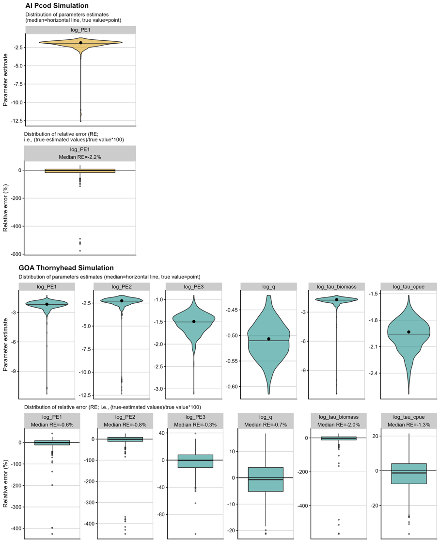Figure 2. Simulation self-test results for AI Pcod (top panels; gold) and GOA Thornyhead (bottom panels; teal). The upper row of each panel gives the distribution of the recovered parameters, with the dot giving the “true value” used to simulate the data. The lower row of each panel gives the relative error of the recovered parameters, with the zero line indicating the simulation returns the “true value,” the box plot line giving the median of the recovered parameter’s relative errors, and the whiskers and dots of the boxplots giving the spread of the recovered parameter’s relative errors.

2. Residual analysis

Residuals are used to test the underlying assumptions about the structure and error distributions in the model. For example, in a linear regression, residuals should be independent, normal, and have constant variance. Traditional residuals (e.g., Pearson’s residuals) are inappropriate for state-space models like REMA, because the random effects induce correlations in the predicted data such that the residuals are no longer independent. Additionally, process error variance may be overestimated in cases where the model is mis-specified, thus leading to artificially small residuals (see Section 3 of Thygesen et al. 2017 for an example). The appropriate residual type for validation of state-space models are one-step ahead (OSA) residuals. Instead of comparing the observed and expected values at the same time step, OSA residuals use forecasted values based on all previous observations (i.e., they exclude the observed value at the current time step from prediction). In this way, OSA residuals account for non-normality and correlation in the residuals among years.

Under a correctly specified model, resultant OSA residuals should be independent and identically distributed (i.i.d.) with a standard normal distribution $N(0,1)$ . This can be tested with a normal QQ plot, where the theoretical quantile values of the standard normal distribution are plotted on the x-axis, and the corresponding empirical quantile values of the OSA residuals are plotted on the y-axis. If the OSA residuals are standard normally distributed, the points will fall on the 0/1 reference line, and the standard deviation of normalized residuals (SDNR) statistic will be close to 1. If the residuals are not standard normally distributed (SDNR far from 1), the points will deviate from the reference line. In the case where the model includes multiple strata and surveys, OSA residuals should be normally distributed within and across strata and surveys, however small sample sizes (e.g., within a single stratum) may not have sufficient statistical power to identify model misfit.

In addition to the normality of OSA residuals, residuals should be random and independent (i.e., they should not be correlated by year). Standard approaches such as autocorrelation function (ACF) plots or residual runs tests (e.g., Wald-Wolfowitz test) are inappropriate for many REMA applications because of missing years of data in the survey time series, and instead, we directly plot the residuals against the years of the survey time series. Visual patterns or extreme outliers (greater than 3 or less than -3 for N(0,1) distribution) in the residuals can indicate structure in the data (i.e., temporal correlation) that is not adequately captured by the model.

Methods for calculating OSA residuals in REMA have been implemented in the rema::get_osa_residuals() using the TMB::oneStepPredict() function and the fullGaussian method when using lognormal error distributions. The rema::get_osa_residuals() returns tidied dataframes of observations, REMA model predictions, and OSA residuals for the biomass and CPUE survey data when appropriate, along with QQ and residual-time series diagnostic plots.

Results of the residual analysis

The normal QQ plot for AI Pcod (Figure 3, top panel) suggests slight negative skewness in the residuals (i.e., the majority of the points fall below the 0/1 line), though the small sample size makes interpretation challenging. The SDNR is 0.99 (recall a perfect model would have an SDNR=1.00), indicating assumptions are likely met for the residuals. The plot of OSA residuals by year (Figure 3, bottom panel) shows no obvious patterns in the residuals, suggesting they are independent; there is no evidence of outliers in the residuals that warrant further inspection.

The combined normal QQ plot for GOA Thornyhead OSA residuals (Figure 4, top panel) suggests they follow a normal distribution (the points fall along the 0/1 line), though there is evidence of slight positive, or right skewness (the majority of the points fall above the 0/1 line). The SDNR is approximately 1, indicating the variance assumptions are likely met for the residuals. The QQ plots for the biomass by strata (Figure 4, middle panels) highlight where some of the positive skewness may be coming from (e.g., EGOA 701-1000m, WGOA 0-500 m); however, small sample sizes by stratum make interpretation of these QQ plots difficult. The QQ plots for the CPUE by strata (Figure 4, bottom panel) are mostly normal, though there is some evidence of light tails in the WGOA stratum.

The plot of OSA residuals by year for the GOA Thornyhead OSA residuals by biomass strata (Figure 5, top panels) show no patterns in the residuals, suggesting they are independent. However, there are runs in the residuals for the CPUE strata (Figure 5, bottom panels), especially in the CGOA and WGOA, which might indicate model misspecification or misfit. There is no evidence of outliers.

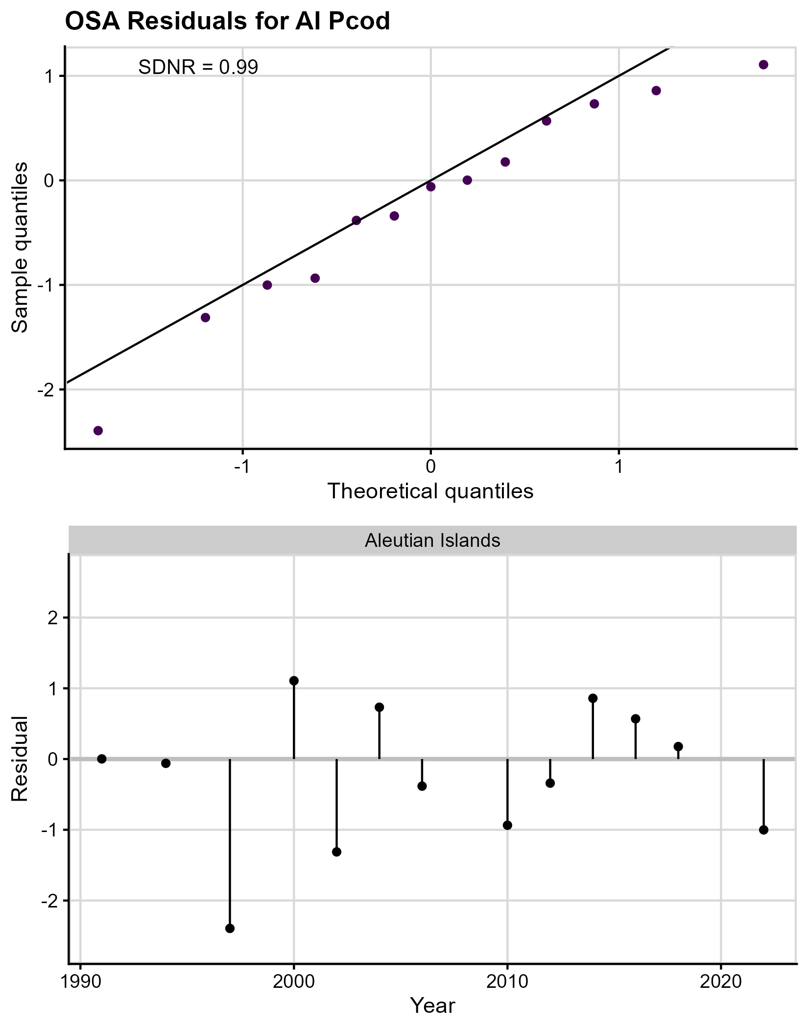Figure 3. One-step ahead (OSA) residual plots for AI Pcod. The top panel gives the QQ plot, comparing the normal distribution quantiles (x-axis) to the OSA residual distribution quantiles (y-axis). The diagonal line is the 0-1 line, where the two quantiles are equal, and the SDNR statistic is given in the upper left of the plot. The bottom panel gives the residuals (y-axis) plotted by year (x-axis) which is used to check for independence.

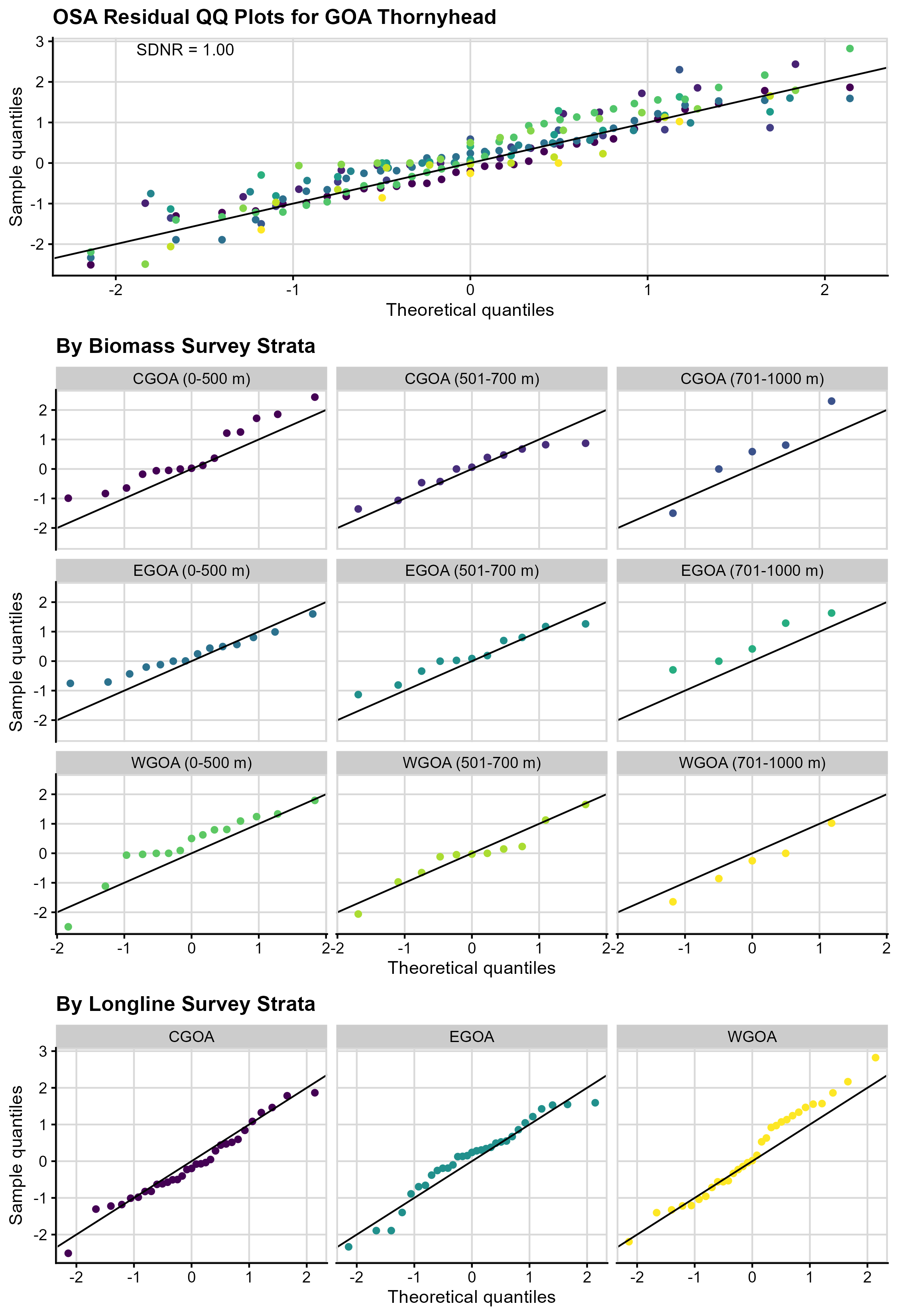Figure 4. One-step ahead (OSA) QQ plots across (top panel) and within strata (middle panel, bottom trawl survey strata; and bottom panel, longline survey strata) for GOA Thornyhead. In both panels, the colors correspond to bottom trawl survey strata. The SDNR statistic is given for the across strata QQ plot; the within strata plots are useful to check for extreme skew but lack statistical power.

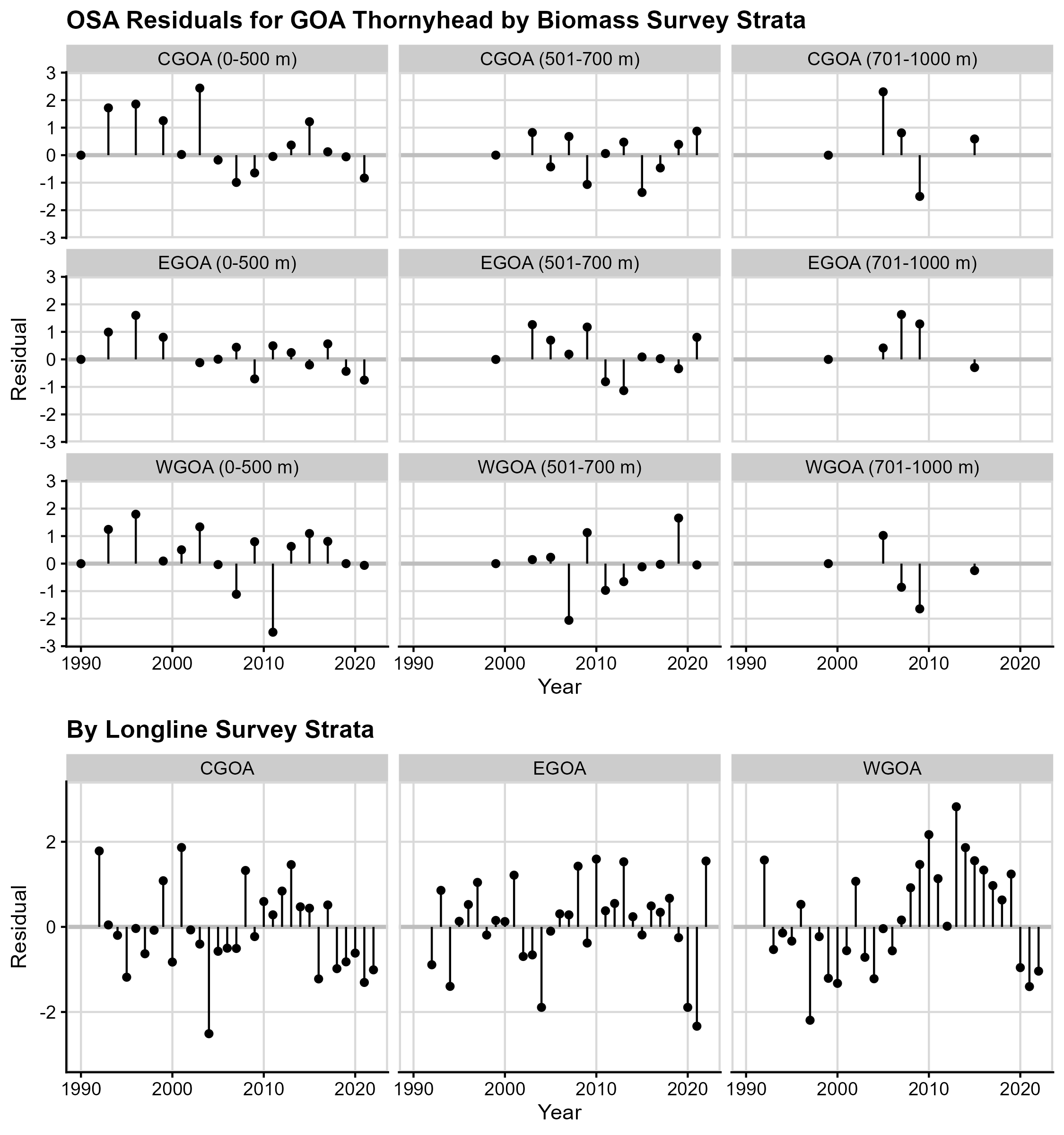Figure 5. One-step ahead (OSA) residual plots for GOA Thornyhead. The residuals (y-axis) for each annual time step (random effect; x-axis) for each survey stratum.

The rema library was developed in Template Model Builder (TMB), which uses maximum marginal likelihood estimation with the Laplace approximation to efficiently estimate high dimensional, non-linear mixed effects models in a frequentist framework (Skaug and Fournier, 2006; Kristensen et al., 2016). The primary assumption in models using the Laplace approximation is that the random effects follow a normal distribution. This assumption simplifies the complex integrals that make up the likelihood function. The Laplace approximation is fast and accurate when the normality assumption is met; however, if the true distribution of the random effects is not normal, the Laplace approximation may introduce bias into the parameter estimates.

We can test the validity of the Laplace approximation using Markov chain Monte Carlo (MCMC) sampling in the tmbstan library, comparing the distributions of the fixed effects parameters from MCMC-sampled models with and without the Laplace approximation (Monnahan and Kristensen, 2018). To do so, we compare the distributions using QQ plots between the two model cases. The Laplace approximation is reasonably accurate if the sampling quantiles for the two models (with and without the Laplace approximation) are similar, i.e., they fall on the 1:1 line. This can also help us identify bias introduced by the Laplace approximation, for example, if the fixed effects estimates and their associated estimates of uncertainty differ between the base model (run with marginal maximum likelihood estimation using the Laplace approximation) and the MCMC versions with and without the Laplace approximation. MCMC models were run with 1000 iterations, assuming a warmup of 500. As discussed in the Results section, iterations were increased to 5000 with a warmup of 2500 for GOA Thornyhead in an effort to improve diagnostics and model convergence.

The function below is used to run the two model cases:

# function to (1) run models with and without laplace approximation for
# comparison and (2) return posterior data frames and models
# function input: model (e.g., AI Pcod or GOA Thornyhead), number of iterations
# (samples), number of chains
mcmc_comp <- function(mod_name, it_numb, chain_numb) {

  # set up MCMC chain information
  it_num <- it_numb
  chain_num <- chain_numb
  # mod_name = pcod_mod; it_num = 1000; chain_num = 4

  # run model with laplace approximation
  mod_la <- tmbstan(obj = mod_name, chains = chain_num, init = mod_name$par, laplace = TRUE, iter = it_num)
  # run model without laplace approximation, i.e., all parameters fully estimated without assumptions of normality
  mod_mcmc <- tmbstan(obj = mod_name, chains = chain_num, init = mod_name$par, laplace = FALSE, iter = it_num)

  # posteriors as data frame
  post_la <- as.data.frame(mod_la); post_la$type <- ("la")
  post_mcmc <- as.data.frame(mod_mcmc); post_mcmc <- post_mcmc[, c(1:length(mod_name$par), dim(post_mcmc)[2])]; post_mcmc$type <- rep("mcmc")
  # informational things... this is for getting the posterior draws, i.e., to
  # test traceplots and such
  post_la$chain <- rep(1:chain_num, each = it_num/2)
  post_la$iter_num <- rep(1:(it_num/2), chain_num)
  post_mcmc$chain <- rep(1:chain_num, each = it_num/2)
  post_mcmc$iter_num <- rep(1:(it_num/2), chain_num)
  post_draws <- rbind(post_la, post_mcmc)

  # get quantiles
  qv <- seq(from = 0, to = 1, by = 0.01)
  quant_dat <- data.frame(quant = NULL,
                          la = NULL,
                          mcmc = NULL,
                          par = NULL)

  for (i in 1:(dim(post_la)[2]-4)) { # post_la has type, chains, lp, iteration number column that don"t count

    tmp <- data.frame(quant = qv,
                      la = quantile(unlist(post_la[i]), probs = qv),
                      mcmc = quantile(unlist(post_mcmc[i]), probs = qv),
                      par = rep(paste0("V", i)))

    quant_dat <- rbind(quant_dat, tmp)

  }

  return(list(quant_dat, post_draws, mod_la, mod_mcmc))

}

# run models
pcod_comp <- mcmc_comp(mod_name = pcod_mod, it_numb = 1000, chain_numb = 3)
thrn_comp_log_tau <- mcmc_comp(mod_name = thrn_mod, it_numb = 5000, chain_numb = 3)

The following code uses the output from mcmc_comp() to make a QQ plot to compare the posterior distributions of the parameters and parameter estimates between the MCMC models with and without the Laplace approximation:

# clean up data frame names by renaming things
pcod_qq <- pcod_comp[[1]]
pcod_qq$par_name <- rep("log_PE1"); pcod_qq$sp <- rep("AI Pcod")
thrn_qq <- thrn_comp_log_tau[[1]]
thrn_qq$par_name <- recode(thrn_qq$par,
                           V1 = "log_PE1",
                           V2 = "log_PE2",
                           V3 = "log_PE3",
                           V4 = "log_q",
                           V5 = "log_tau_biomass",
                           V6 = "log_tau_cpue")
thrn_qq$sp <- rep("GOA Thornyhead")
qq_dat <- rbind(pcod_qq, thrn_qq)

# plot
plot_laplace_mcmc <- function(qq_dat, plot_title) {
  ggplot(qq_dat, aes(mcmc, la)) +
    geom_abline(intercept = 0, slope = 1, col = "lightgray") +
    geom_point() +
    facet_wrap(~par_name, scales = "free", nrow = 2,  dir = "v") +
    labs(x = "MCMC", y = "Laplace approx.", title = plot_title) +
    theme(plot.title = element_text(size = 12),
          axis.text = element_text(size = 7),
          axis.title = element_text(size = 11),
          strip.text = element_text(size = 11))
}
p1 <- plot_laplace_mcmc(pcod_qq, "AI Pcod")
p2 <- plot_laplace_mcmc(thrn_qq, "GOA Thornyhead")
cowplot::plot_grid(p1, p2, rel_widths = c(0.4,0.6), ncol = 2)
ggsave(paste0("vignettes/ex4_mcmc_qq.png"), width = 11, height = 7, units = "in", bg = "white")

# parameter summary table - compare the marginal max likelihood estimates (MMLE)
# with the mcmc estimates. Rhat is the potential scale reduction factor on split
# chains (at convergence, Rhat=1)
m <- summary(pcod_comp[[3]])$summary[1, c(6,4,8,10), drop = FALSE]
psum <- data.frame(Stock = 'AI Pcod', Model = 'MCMC_Laplace', FixedEffect = row.names(m), m, row.names = NULL)
m <- summary(pcod_comp[[4]])$summary[1, c(6,4,8,10), drop = FALSE]
psum <- psum %>% bind_rows(data.frame(Stock = 'AI Pcod', Model = 'MCMC_withoutLaplace', FixedEffect = row.names(m), m, row.names = NULL))
m <- summary(thrn_comp_log_tau[[3]])$summary[1:6, c(6,4,8,10), drop = FALSE]
psum <- psum %>% bind_rows(data.frame(Stock = 'GOA Thornyhead', Model = 'MCMC_Laplace', FixedEffect = row.names(m), m, row.names = NULL))
m <- summary(thrn_comp_log_tau[[4]])$summary[1:6, c(6,4,8,10), drop = FALSE]
psum <- psum %>% bind_rows(data.frame(Stock = 'GOA Thornyhead', Model = 'MCMC_withoutLaplace', FixedEffect = row.names(m), m, row.names = NULL))
pars <- as.list(pcod_mod$sdrep, "Est")$log_PE
sd <- as.list(pcod_mod$sdrep, "Std")$log_PE
psum <- psum %>% bind_rows(data.frame(Stock = 'AI Pcod', Model = 'Base_MMLE_Laplace', FixedEffect = "log_PE",
                                      X50. = pars, X2.5. = pars-1.96*sd, X97.5. = pars+1.96*sd, Rhat = NA))
pars <- unlist(as.list(thrn_mod$sdrep, "Est"))
pars <- pars[names(pars)[grepl("log_PE|log_q|log_tau", names(pars))]]
sd <- unlist(as.list(thrn_mod$sdrep, "Std"))
sd <- sd[names(sd)[grepl("log_PE|log_q|log_tau", names(sd))]]
psum <- psum %>% bind_rows(data.frame(Stock = 'GOA Thornyhead', Model = 'Base_MMLE_Laplace', FixedEffect = rownames(summary(thrn_comp_log_tau[[3]])$summary[1:6,,drop=FALSE]),
                                      X50. = pars, sd = sd, row.names = NULL) %>%
                             mutate(X2.5. = X50.-1.96*sd,
                                    X97.5. = X50.+1.96*sd,
                                    Rhat = NA) %>%
                             select(-sd))
# write.csv(psum, 'vignettes/ex4_param_table.csv')

Results for testing the validity of the Laplace approximation

Figure 6 gives the compared quantiles from full MCMC testing (x-axis) and the Laplace approximation (y-axis) for AI Pcod and GOA Thornyhead models.

For the simpler AI Pcod model (Figure 6, left panel), the Laplace approximation and full MCMC testing show a similar distribution, indicating that the Laplace approximation is reasonable. Additionally the estimates of fixed effects are nearly identical between the base model and MCMC models with and without the Laplace approximation (Table 1).

For the more complex GOA Thornyhead model, the preliminary model results based on 1000 iterations exhibited poor diagnostics for all process error parameters and the additional observation error for the biomass survey (log_tau_biomass). We increased the number of MCMC iterations to 5000 in an effort to improve convergence diagnostics; however, the log_tau_biomass parameter continued to show significant deviations between the models with and without the Laplace approximation (Figure 6, right panels). A comparison of the fixed effects estimates between the base models show large differences in the parameter estimates and their associated estimates of uncertainty (Table 1). This indicates that the Laplace approximation is likely inaccurate, and that further investigation into model structure might be necessary.

Table 1. AI Pcod and GOA Thornyhead fixed effect estimates with 95% confidence or credible intervals for maximum likelihood or MCMC models, respectively (CI). Fixed effects estimates are compared between the base model run with marginal maximum likelihood estimation assuming the Laplace approximation (“Base_MMLE_Laplace”) and MCMC models with and without the Laplace approximation (“MCMC_Laplace” and “MCMC_withoutLaplace”, respectively). The Rhat statistic is provided for MCMC models and is a convergence metric (convergence = Rhat = 1). Nonconverged parameters are highlighted in bold. The parameter estimate for the MCMC models is the median of the posterior samples.

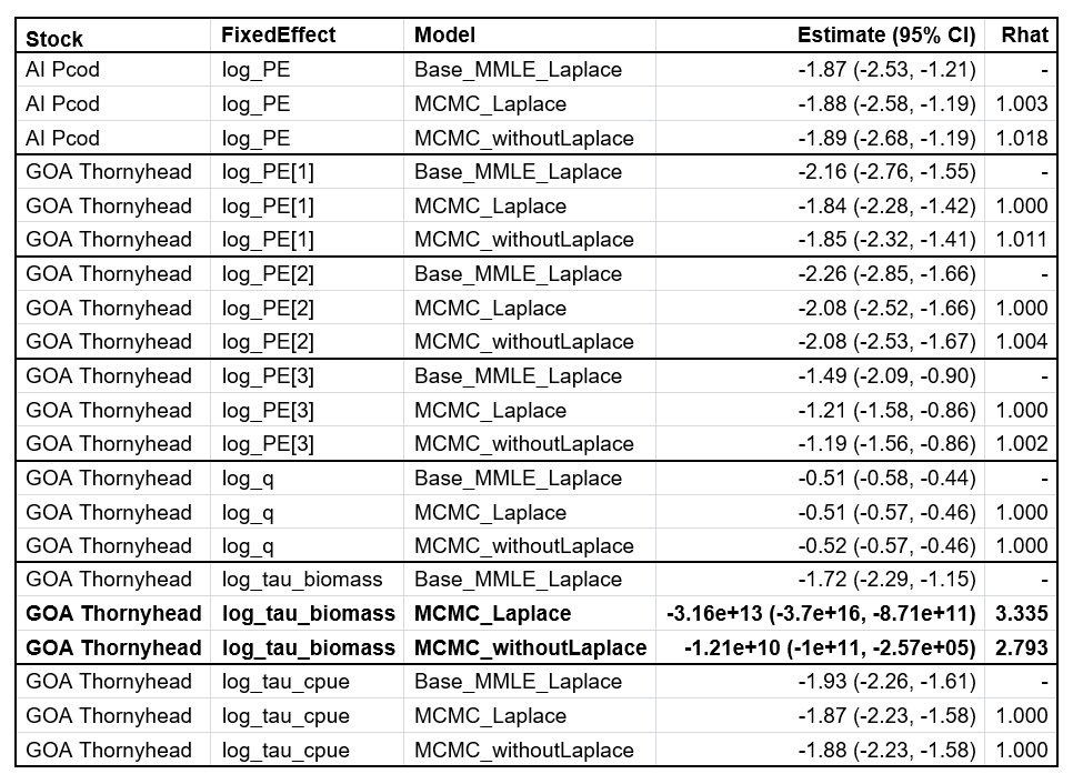
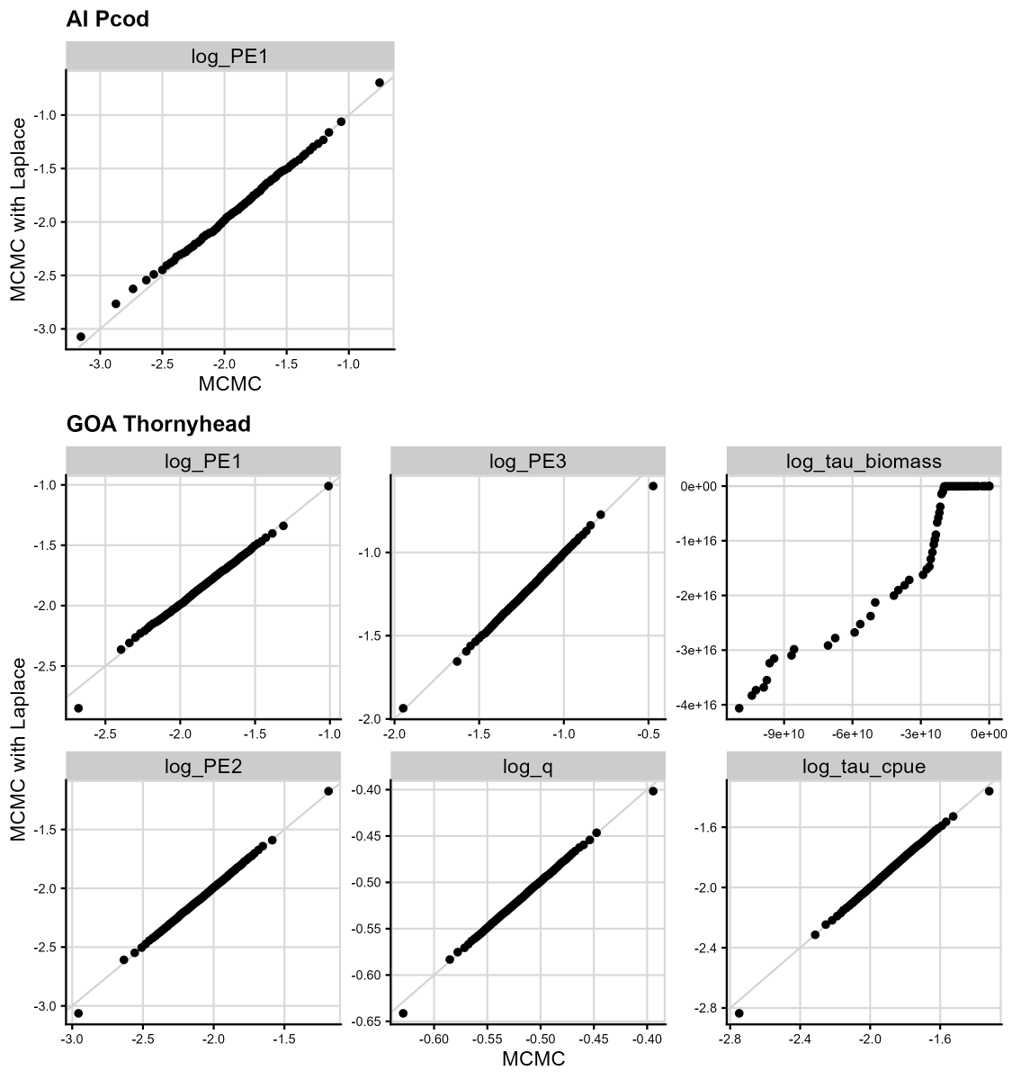
Figure 6. Results from Laplace approximation testing. We compare the results of running a model without assuming normality of random effects (MCMC, x-axis) and running a model assuming normality of random effects (Laplace approximation, y-axis), where the quantiles of each are plotted against each other for each fixed effect in the model. The gray line is the 1:1 line; points that fall on the gray line indicate that the quantile value is the same between the two cases. The top panel gives the plot for the AI Pcod model (one fixed effect), and the bottom panels give the plots for the GOA Thornyhead model (six fixed effects).

4. Parameter correlation: Are the model parameters identifiable and non-redundant?

Parameter redundancy refers to the idea that multiple parameters contribute to the model in the same way. An intuitive case is $y \sim \beta_1 + \beta_2 + \alpha x$ , since the model could estimate many combinations of $\beta_1$ and $\beta_2$ which minimize the log-likelihood, i.e., the sampled parameters will be correlated. To reduce redundancy, $\beta_1 + \beta_2$ can be redefined as $\beta_0$ .

Results of parameter correlation analysis

Figure 7 shows a pairwise correlation matrix of the posterior draws for the GOA Thornyhead model (the MCMC model with the Laplace approximation), with histograms of the univariate marginal distributions on the diagonal and a scatterplot of the bivariate distributions off the diagonal. There are significant unresolved sampling problems of the log_tau_biomass parameter, shown by the non-normal and heavily skewed distribution of log_tau_biomass. The pairwise scatterplots on the off-diagonals show that the heavy left tails in log_tau_biomass are causing interactions (i.e., correlation) with almost all other parameters in the model. This diagnostic is a clear indication that there is model mis-specification that warrants further investigation.

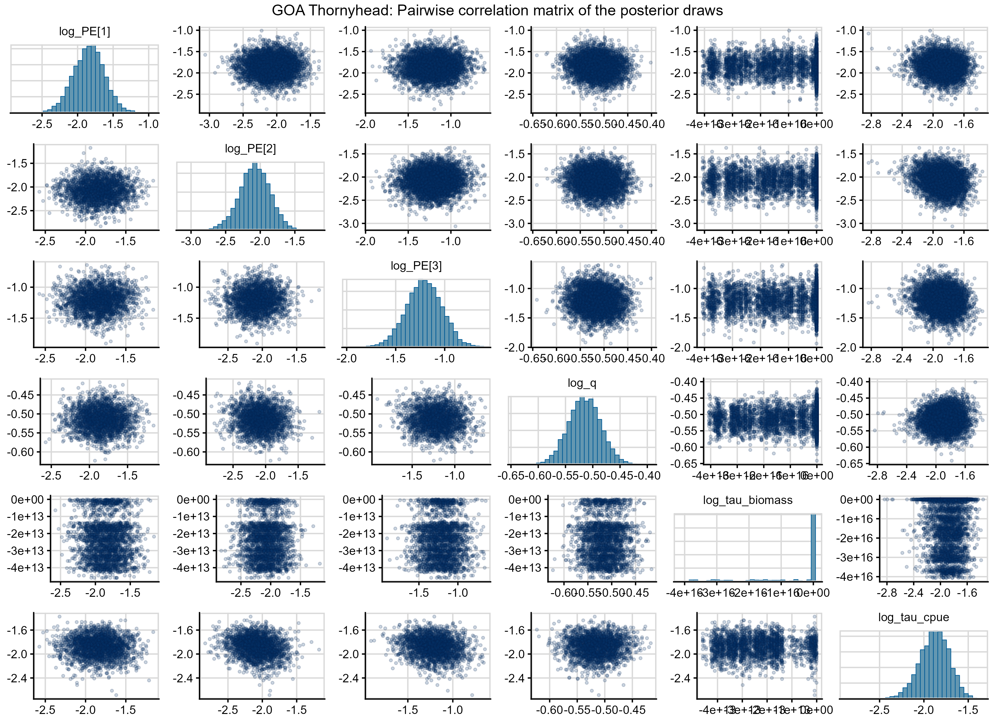
Figure 7. Pairs plot for the GOA Thornyhead MCMC model assuming the Laplace approximation. The diagonal plots give the distribution of each fixed effect for 2500 MCMC draws. The off-diagonal elements give the parameter-by-parameter correlation, where each point gives the parameter values estimated from the same MCMC simulation.

5. Is the GOA Thornyhead model really converged?

Despite the poor diagnostics shown in this vignette for the GOA Thornyhead model, the standard output in TMB and rema suggests that this model is converged (i.e., it has a low maximum gradient component and the standard error estimates appear reasonable). Within the MCMC framework, we can look at the mixing of MCMC across multiple chains using a diagnostic called a traceplot to assess convergence. The following code shows how to do that within the rstan library (Stan Development Team, 2024):

p1_mcmc_pcod <- rstan::traceplot(pcod_comp[[3]]) + ggtitle(label = "Traceplots to assess mixing across Markov chains and convergence", subtitle = "AI Pcod")
p1_mcmc_thrn <- rstan::traceplot(thrn_comp_log_tau[[3]], ncol = 3) + ggtitle(label = NULL, subtitle = "GOA Thornyhead")
cowplot::plot_grid(p1_mcmc_pcod, p1_mcmc_thrn, ncol = 1)
ggsave(paste0("vignettes/ex4_traceplots.png"), width = 11, height = 8, units = "in", bg = "white")

From the traceplots for both models in the figures below, we see that the AI Pcod model MCMC chains are fully mixed and the model is converged (top panel). However, for the GOA Thornyhead model (bottom panel), we see that the estimation of additional observation error (log_tau_biomass) is causing convergence issues and the MCMC chains are not well mixed.

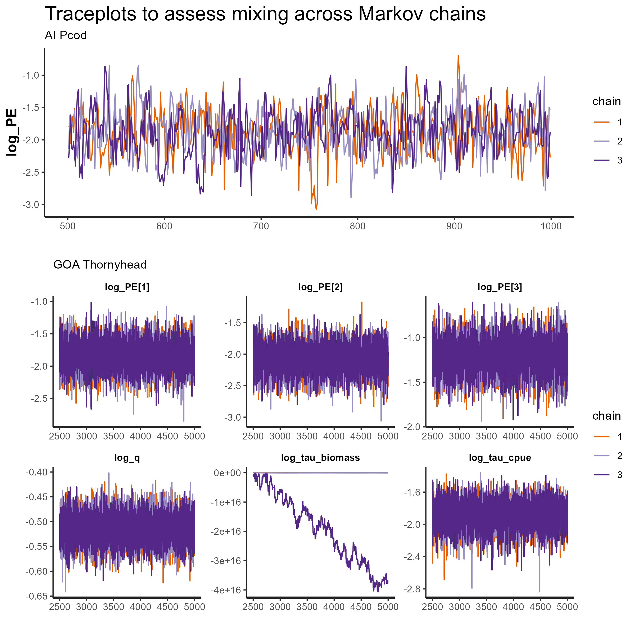
Figure 8. MCMC traceplots for AI Pcod (top panel) and GOA Thornyhead (bottom panels). Each subpanel is an individual parameter, and the plot gives the value of the parameter (y-axis) for each simulation draw (x-axis) for each model chain (color).

When should we care about failed model diagnostics?

The REMA model is used within the NPFMC to obtain exploitable biomass estimates for Tier 4 crab and Tier 5 groundfish and as a method to apportion Acceptable Biological Catches among management regions (Sullivan et al., 2022). So then, if its primary purpose is to smooth noisy survey biomass estimates (i.e., if we are using it as a fancy average), do we need to care about potential red flags raised during model validation?

Yes: In the case of the GOA Thornyhead model, for example, it appears there is an issue with the estimation of the additional observation error, pointing to potential over-parameterization of the model and/or parameter redundancy. Because terminal year predictions from the REMA model are the quantities directly used for management, and the estimation of additional observation error by definition increases the “smoothness” of model predictions, the answer is likely yes in this particular case.
Maybe not: In a hypothetical case where the estimation of year predictions show no diagnostic concerns, but uncertainty estimations show possible diagnostic problems, model validation red flags might be less important. This is because uncertainty results from REMA are not generally used for fisheries management at the NPFMC. In other words, failed model validation criteria are primarily a concern when they impact the quantities of interest in the model (in our case, biomass predictions). Model validation, and subsequent interpretation, should be considered in light of the goal of the model, rather than as a binary pass/fail testing procedure.

Preliminary recommendations

The model validation methods presented here are tools for stock assessment scientists to evaluate existing models and guide development of future models. From this analysis, we found that the REMA model can recover parameters across the range of complexity relevant to NPFMC Tier 4 and Tier 5 stocks. Our analysis suggests that the MCMC diagnostics and OSA residuals to be the most useful diagnostics for the REMA model. When models fail these diagnostics, it may indicate that the model is too complex and simplifications should be considered. We have highlighted several places in this document how diagnostic features can help make choices about the most appropriate model simplifications (pool process errors, remove additional observation errors, etc.) in light of REMA model assumptions and trade-offs between model parameters. Our results indicate that these diagnostics are most important to explore for existing models using multivariate configurations with multiple process errors, multi-survey versions using CPUE indices like the longline survey, and models estimating additional observation error. While model validation may not be needed for all existing REMA models, we recommend they be used when recommending new models for management.

References

Aeberhard, W.H., Flemming, J.M., Nielsen, A. 2018. Review of State-Space Models for Fisheries Science. Annual Review of Statistics and Its Application, 5(1), 215-235. https://doi.org/10.1146/annurev-statistics-031017-100427

Auger-Méthé, M., Field, C., Albertsen, C.M., Derocher, A.E., Lewis, M.A., Jonsen, I.D., Flemming, J.M. 2016. State-space models’ dirty little secrets: even simple linear Gaussian models can have estimation problems. Scientific reports, 6(1), 26677.

Auger‐Méthé, M., Newman, K., Cole, D., Empacher, F., Gryba, R., King, A. Leos-Barajas, V., Flemming, J.M., Nielsen, A, Petris, G., Thomas, L. 2021. A guide to state–space modeling of ecological time series. Ecological Monographs, 91(4), e01470.

Campbell, D., & Lele, S. 2014. An ANOVA test for parameter estimability using data cloning with application to statistical inference for dynamic systems. Computational Statistics & Data Analysis, 70, 257-267.

Cole, D. J. 2019. Parameter redundancy and identifiability in hidden Markov models. Metron, 77(2), 105-118.

Echave, K.B., Siwicke, K.A., Sullivan, J., Ferriss, B., and Hulson, P.J.F. 2022. Assessment of the Thornyhead stock complex in the Gulf of Alaska. In Stock assessment and fishery evaluation report for the groundfish fisheries of the Gulf of Alaska. North Pacific Fishery Management Council, 605 W. 4th. Avenue, Suite 306, Anchorage, AK 99501. https://apps-afsc.fisheries.noaa.gov/Plan_Team/2022/GOAthorny.pdf

Gabry, J. and Mahr, T. 2024. bayesplot: Plotting for Bayesian Models. R package version 1.11.1, https://mc-stan.org/bayesplot/.

Gabry, J., Simpson, D., Vehtari, A., Betancourt, M., Gelman, A. 2019. Visualization in Bayesian workflow. J. R. Stat. Soc. A. (182) 389-402. doi:10.1111/rssa.12378 https://doi.org/10.1111/rssa.12378.

Kristensen, K., Nielsen, A., Berg, C.W., Skaug, H., Bell, B.M. 2016. TMB: Automatic differentiation and Laplace approximation. J Stat Softw. 2016; 70(5):21. Epub 2016-04-04. https://doi.org/10.18637/jss.v070.i05

Monnahan, C.C., & Kristensen, K. 2018. No-U-turn sampling for fast Bayesian inference in ADMB and TMB: Introducing the adnuts and tmbstan R packages. PloS one, 13(5), e0197954.

Skaug, H.J., and Fournier, D.A. 2006. Automatic approximation of the marginal likelihood in non-Gaussian hierarchical models. Computational Statistics & Data Analysis, 51(2), 699-709.

Spies, I., Barbeaux, S., Hulson, H., Ortiz, I. 2023. Assessment of the Pacifc cod stock in the Aleutian Islands. In Stock assessment and fishery evaluation report for the groundfish fisheries of the Bering Sea and Aleutian Islands. North Pacific Fishery Management Council, 605 W. 4th. Avenue, Suite 306, Anchorage, AK 99501. https://apps-afsc.fisheries.noaa.gov/Plan_Team/2023/AIpcod.pdf

Stan Development Team. 2024. RStan: the R interface to Stan. R package version 2.32.6, https://mc-stan.org/.

Sullivan, J., Monnahan, C. Hulson, P. Ianelli, J. Thorson, J. Havron, A. 2022. REMA: A consensus version of the random effects model for ABC apportionment and Tier 4/5 assessments. Plan Team Report, Joint Groundfish Plan Teams, North Pacific Fishery Management Council. 605 W 4th Ave, Suite 306 Anchorage, AK 99501. Available through the Oct 2022 Joint GPT e-Agenda.

Thygesen, U.H., Albertsen, C.M., Berg, C.W., Kristensen, K., & Nielsen, A. 2017. Validation of ecological state space models using the Laplace approximation. Environmental and Ecological Statistics, 24(2), 317-339. https://doi.org/10.1007/s10651-017-0372-4

Laurinne J Balstad, Jane Sullivan, and Cole Monnahan